Workshop 5 Worksheet

Learning outcomes

By the end of the session, you should:

gain practice interpreting inferential statistics in regression outputs
progress with the analysis required for your chosen assignment question

Intro

So far, in all previous exercises, we paid almost exclusive attention to obtaining “point estimates” for our independent (explanatory, predictor) variables. These “point estimates” tell us the average and constant effect that a one-unit change in the predictors have on the outcome (dependent) variable, and do so with seemingly unashamed confidence, despite the fact that, as we have seen in some cases (e.g. Portugal’s trust score), they predict individual data points rather poorly.

In Exercise 3.2 we addressed the research question “How is income inequality (at national level) associated with social trust when we adjust for the potential influence of homicide rates?”, but we focused almost exclusively on interpreting the coefficient estimates we obtained for the two predictor variables (\(-7.147\) for Income inequality and \(0.174\) for Homicides. You should by now be able to confidently interpret these coefficients; if not, you can return to and consult the detailed explanation given in Exercises 3.1-3.

But we did not focus at all on some of the other statistics from these models, which could tell us more about how variable (i.e. precise) these estimates are, and what is the probability that these coefficients obtained from relatively small samples can tell us something reliable about the associations/effects we should find in the whole true population from which these samples were drawn?

We are already given two of these in the standard default output in the columns “Standard Error” and “p”. Another useful such statistic – which relates to both of the previously mentioned ones and is often a more descriptive option –, is the “95% Confidence Intervals”, which is not shown by default but can be requested in the Statistics drop-down options set:

Figure 1: Multiple linear regression in JASP (including 95% Confidence Intervals)

Similarly, in Exercise 4.1.1 we addressed the research question How did sex-adjusted age shape social trust in Britain in 2010-2011? using the 2010 British Social Attitudes survey (gb-bsa10-trust.sav), and we fit a logistic regression model that estimated the effect of Age to be \(0.006\) “log-odds” (an odds ratio of \(1.006\) ) and the effect of being a woman as opposed to being a man (Sex (Female)) to be \(-0.437\) “log-odds” (an odds ratio of \(0.646\)). We also plotted these estimates/coefficients on the probability scale to get a more intuitive understanding of what they actually mean. You should by now be able to interpret these coefficients with some confidence; if not, you can return to and consult the detailed explanation given in Exercise 4.1.1. Again, however, we did not focus at all on the statistics shown in the “Standard Error” and “p” columns. We can also request the “95% Confidence Interval” in the Statistics drop-down options set, just like in the case of linear regression; for logistic regression we also have the option to request the confidence intervals for either the “Estimate” (i.e. the point estimate, similar to what in the case of linear regression in labelled by JASP as the “Unstandardized” coefficient) or for the “Odds Ratio”:

Figure 2: Multiple logistic regression in JASP (including 95% Confidence Intervals)

Which of the options we prefer will depend on which of the two we prefer to interpret in more detail in writing; as we discussed, neither are particularly intuitive for human brains, but often the Odds Ratio can provide a clearer interpretation as a percentage change in the odds of being in the indicator outcome category (the one coded as “1”) as opposed to being in the other - reference - category. So you will often see results reported in Odds Ratios in publish articles.

Exercise 5.1: Interpreting inferential statistics

This first exercise is purely conceptual: focus on these statistics relating to the precision and the inferential reliability of the estimates obtained from the two multiple regression models above and try to interpret them in writing.

Questions

Using the lecture slides and the assigned readings, interpret the results focusing on the meaning of the “Standard Error”, “95% CI” and “p” columns

Solution: bringing it all together

Once we have thought about the precision and the inferential reliability of the estimates obtained from our models, we can summarise our statistical findings concisely. We could describe our findings in these words:

As we can see in Figure 1, a multiple linear regression model has shown that while adjusting for the level of Homicides in a given country, Income inequality is negatively associated with Trust. The model estimates that a one-unit increase in Income inequality is associated with a \(7.147\)-point average decrease in social trust as measured on the Trust scale. This estimate can be taken as statistically significant (p-value \(< 0.001\)), with a 95% Confidence Interval ranging from \(-11\) to \(-3.3\). The rate of Homicides, however, proved not to be a statistically significant predictor of Trust (\(p=0.483\), \(\text{95% CI}=-0.33 \text{ to } 0.68\)) when adjusting for the effect of Income inequality.

Or:

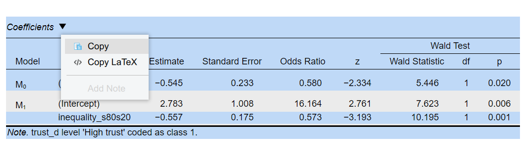
We fit a multiple logistic regression model to estimate the joint effect of Age and Sex of trust. The results are shown in Figure 2. We find that, whilst adjusting for the effect of all the other explanatory variables in the model, a positive difference of one year in one’s Age is associated with a \(0.6\%\) higher odds of thinking that “most people can be trusted”. However, our 95% Confidence Interval can vary between \(0\%\) and \(1.3\%\), and therefore we cannot exclude the possibility that our estimate is due purely to chance, which is confirmed by the p-value of \(0.07\). We cannot, therefore, be confident that our estimate is correct for the wider population. On the other hand, being a female - as opposed to being a male - is statistically significantly (\(p<0.001\)) associated with a \(35.4\%\) decrease in the odds of thinking that “most people can be trusted” (OR = \(0.646\), 95% CI = \(0.505\) to \(0.825\)). Put differently, men have a higher probability of trusting other than women do, when adjusting for Age.

Exercise 5.2. Complete your analysis for Assignment 2

You will find a detailed guide for Assignment 2 on Canvas, which outlines all the steps involved in completing the assignment, including the recommended structure of the final report

In this exercise, you will focus on the analysis component of the assignment which you can then expand or change if your literature review and interpretation of the results necessitate it.

Once you have chosen your preferred research question from among the listed ones and identified the dataset you will want/need to use to address the question, you can follow the basic steps of the data analysis cycle, which we have also tried to follow in the exercises in the previous two workshops:

Identify the variables you want to use and provide some summary descriptive statistics for them; (this was the topic of Workshop 1)
Check some more detailed univariate descriptive tabulations and/or visualisations of the core variables (at least the outcome variable and the main explanatory variable); (this was the topic of Workshop 1)
Identify and perform any required data cleaning and transformations (e.g. rename variables to more human-readable names, set additional missing values, label and recode categories, reverse, centre or standardise scales); (we did variable transformations as part of exercises in Workshops 3 and 4).
Explore some initial bivariate descriptive tabulations and/or visualisations of the core variables (at least between the outcome variable and the main explanatory variable); (this was the topic of Workshop 2)

↺ Identify and perform any additionally required data cleaning and transformations, and return to Step 3
Fit a simple bivariate regression model to test the unadjusted statistical association/relationship between the outcome variable and the main explanatory variable); (this was the topic of Workshops 3 and 4, depending on which regression method (linear or logistic) your dependent variable requires)

↺ Identify and perform any additionally required data cleaning and transformations, and return to Step 3
Build a multiple regression model to test the partial statistical association/relationship between the outcome variable and the main explanatory variable adjusted for the effect of a number of other independent/control/explanatory variables; (this was the topic of Workshops 3 and 4, depending on which regression method (linear or logistic) your dependent variable requires)

↺ Identify and perform any additionally required data cleaning and transformations, and return to Step 3
Provide a comprehensive but concise statistical interpretation of the regression results: (a) the direction and strength of the relationships, (b) the explanatory strength of the model, (c) the reliability and generalisability of the model estimates; (this is the topic of this week’s lecture and Exercise 5.1 above).

You will perform these analysis steps in JASP, following which you will:

write down your interpretation of your results in as much detail as possible (either (or both) In JASP notes and your main Word/Text editor document that you are using to write the main text of the report in; it’s a good idea to start saving your notes and interpretations alongside the analysis and outputs directly in JASP to make your work reproducible, then copy it over and adapt it in your main document;
Select which outputs (descriptive tables, graphs, statistical output tables) you will want to include in the main text of your report and copy them over from JASP into your Word document/text editor. To copy and paste outputs from JASP, you can click on the small black down-arrows next to the output and select “Copy”, then paste it into your text editor. (Keep in mind that tables will require some manual improvements in Word/text editor to make the content fit the page well).

Make sure to give a caption/title to your graphs and tables in your report.
Identify the main limitations of the statistical analysis and discuss how they could be improved with more appropriate measurements and statistical techniques;
Provide a sociological discussion of how the statistical results, acknowledging the limitations of the analysis, contribute to addressing the research question.