Workshop 4 Worksheet
Learning outcomes
By the end of the session, you should be familiar with:
- running logistic regression in JASP
- the interpretation of logistic regression coefficients
- sub-setting/filtering data in JASP
- recoding/dichotomising a variable in JASP
Intro
This workshop introduces another type of regression analysis: binary/binomial “logistic” or ”logit” regression. Binary logistic regression allows us to model dependent (”response”, “outcome”) \(y\) variables that are not measured on a continuous numeric scale, but instead on a simple dichotomous scale that allows only two values (e.g. “1”/“0”; “Yes”/“No”; “True”/“False”; “Present”/“Abstent”; “Success”/“Failure”; “Agree”/“Disagree”; “Trusts”/“Doesn’t trust”; “Survived”/“Didn’t survive”, etc.). Such a variable is called dichotomous because its two value options present a “dichotomy”, but it is also often referred to by other names: binary or binomial (because it can take only two mutually exclusive values), indicator (because it “indicates” membership in a category - usually the category with the “positive” logical connotation (i.e. “yes”, “true”, “survived”, “trusts”, etc.), coded as 1) or “dummy” (from the word’s meaning of a substitute or a proxy - as in “crash-test dummy” as a substitute for a human) - to signal the variable’s role as a placeholder that indicates the presence (typically coded as 1) or absence (coded as 0) of a specific qualitative characteristic. I will be using these terms interchangeably, depending of the context, just to confuse you (and because these terms are all used in the published literature, which can be confusing).
Modelling such a variable using the linear regression approach from Workshop 3 is likely to result in inaccurate coefficients, because linear regression assumes a theoretically unbounded continuous numeric scale of measurement; when it encounters a binary outcome variable, it assumes that we only observed two values (0 and 1) on this unbound scale, but that the scale nevertheless exists in theory and other values could have been observed if we collected more data. But, in fact, we know that no other values are theoretically possible.
Nevertheless, we can generalise the logic of linear regression to make it applicable to dichotomous dependent variables. In fact, the method we learn about today - binary/binomial logistic regression - is an elementary case of a broader category of statistical models called generalised linear models (GLMs). GLMs can be thought of as a two-stage modelling approach, in which we first model the response variable using a probability distribution - such as the binomial distribution in our case -, and then we model the parameter of the distribution using a collection of predictors and a special form of multiple regression. In essence, with binary logistic regression we will attempt to predict the probability that an observation falls into one of the two categories of a dichotomous dependent (outcome) variable based on one or more independent (predictor, explanatory) variables. Observations are predicted to fall into whichever one of the two outcome categories is most probable for them given the values they have on the independent variable(s). Logistic modelling is thus often considered a classification method, especially in machine learning parlance.
This all sounds very technical and it does involve some complex mathematics, but applying logistic regression in practice will feel very similar to what we have done with linear regression before. The challenge will be in finding the simplest way to interpret the statistical results accurately and meaningfully given that the resulting regression coefficients refer to estimates on a mathematically transformed scale rather than the original scale of measurement of the variables as it was the case in linear regression.
The Advanced topics readings assigned for this week outline these challenges for those who would like to gain a deeper understanding of the mathematics and mechanics of logistic regression; for the rest of us, Connelly, Gayle, and Lambert (2016) (on the reading list) provides a very approachable introduction to the major challenges, specifically for sociological analyses (see, specifically, the sections between Parameter estimates in logistic regression models and The presentation of logistic regression results).
In the exercises below, we return to some of the small individual-level datasets we used in Workshop 1 and 2, which contain selected variables from the British Social Attitudes Survey, the Citizenship Survey and the Community Life Survey (find them under the Questions of Trust tab on the Data page).
The exercises will also allow us (require?) to practice some basic data transformation techniques in JASP that may come useful for the assignment work too (such as renaming, filtering, reordering, recoding/computing variables, and setting custom missing values). This will take us an important step closer to being able to follow the ten basic steps of the data analysis cycle, which are also the ones that will structure your assignment reports:
Identify the variables you want to use and provide some summary descriptive statistics for them;
Check some more detailed univariate descriptive tabulations and/or visualisations of the core variables (at least the outcome variable and the main explanatory variable);
Identify and perform any required data cleaning and transformations (e.g. rename variables to more human-readable names, set additional missing values, label and recode categories, reverse, centre or standardise scales);
Explore some initial bivariate descriptive tabulations and/or visualisations of the core variables (at least between the outcome variable and the main explanatory variable);
↺ Identify and perform any additionally required data cleaning and transformations, and return to Step 3
Fit a simple bivariate regression model to test the unadjusted statistical association/relationship between the outcome variable and the main explanatory variable);
↺ Identify and perform any additionally required data cleaning and transformations, and return to Step 3
Build a multiple regression model to test the partial statistical association/relationship between the outcome variable and the main explanatory variable adjusted for the effect of a number of other independent/control/explanatory variables;
↺ Identify and perform any additionally required data cleaning and transformations, and return to Step 3
Provide a comprehensive but concise statistical interpretation of the regression results: (a) the direction and strength of the relationships, (b) the explanatory strength of the model, (c) the reliability and generalisability of the model estimates;
Identify the main limitations of the statistical analysis and discuss how they could be improved with more appropriate measurements and statistical techniques;
Provide a sociological discussion of how the statistical results, acknowledging the limitations of the analysis, contribute to addressing the research question.
Exercise 4.1: How did sex-adjusted age shape social trust in Britain in 2010-2011?
There is a lot of specificity built into this question. Let’s break it down:
- we want to understand what/how some social factors “shape social trust”: in other words, we need some data measuring social trust in some way and we will want to model that social trust variable (i.e. treat it as our dependent variable, as the “explanandum”, the phenomenon that needs to be explained);
- “sex-adjusted age”: this tells us that the social factors we are interested in using as explanatory variables; we are primarily interested in the effect of “age” on “social trust”, but we want to ensure that we eliminate from that equation any potential influence of biological “sex”. This tells us that we will need to apply a multiple regression model that can consider the combined effect of two or more explanatory variables;
- “Britain in 2010-2011” tells us that we need to find data from Great Britain collected around the years 2010/2011.
What the question doesn’t tell us is:
- what measurement “type” will the “social trust” variable have, and consequently what kind of multiple regression we will have to use.
This is the kind of close reading that you need to apply to the assignment questions too: they have a lot of “specificity” built into them, but at the same time they leave many aspects open to the analyst’s (you) interpretation and choices.
To address this question, we have more than one option when it comes to data sources. We will try out two: the (reduced, toy version of the) 2010 British Social Attitudes Survey (gb-bsa10-trust.sav) and the 2010/2011 Citizenship Survey (gb-cs10-trust.sav).
Exercise 4.1.1. British Social Attitudes Survey, 2010
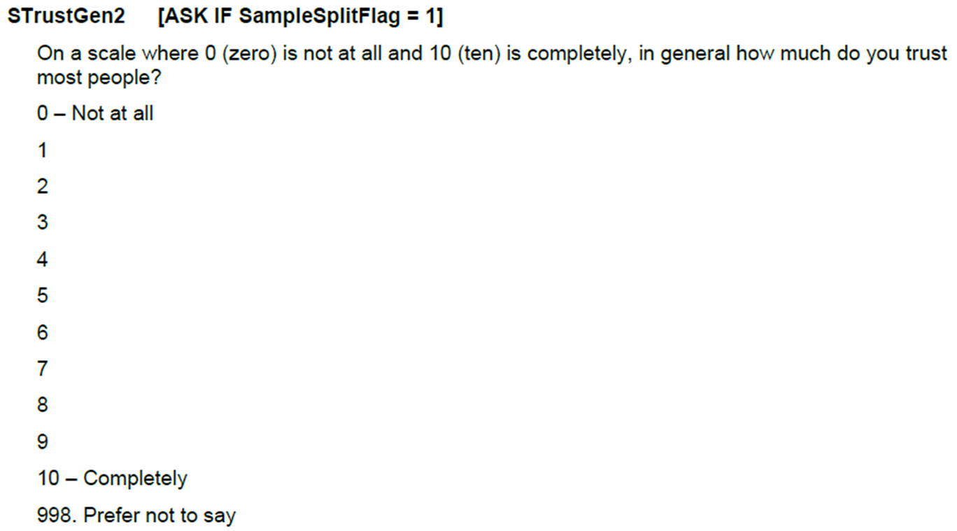
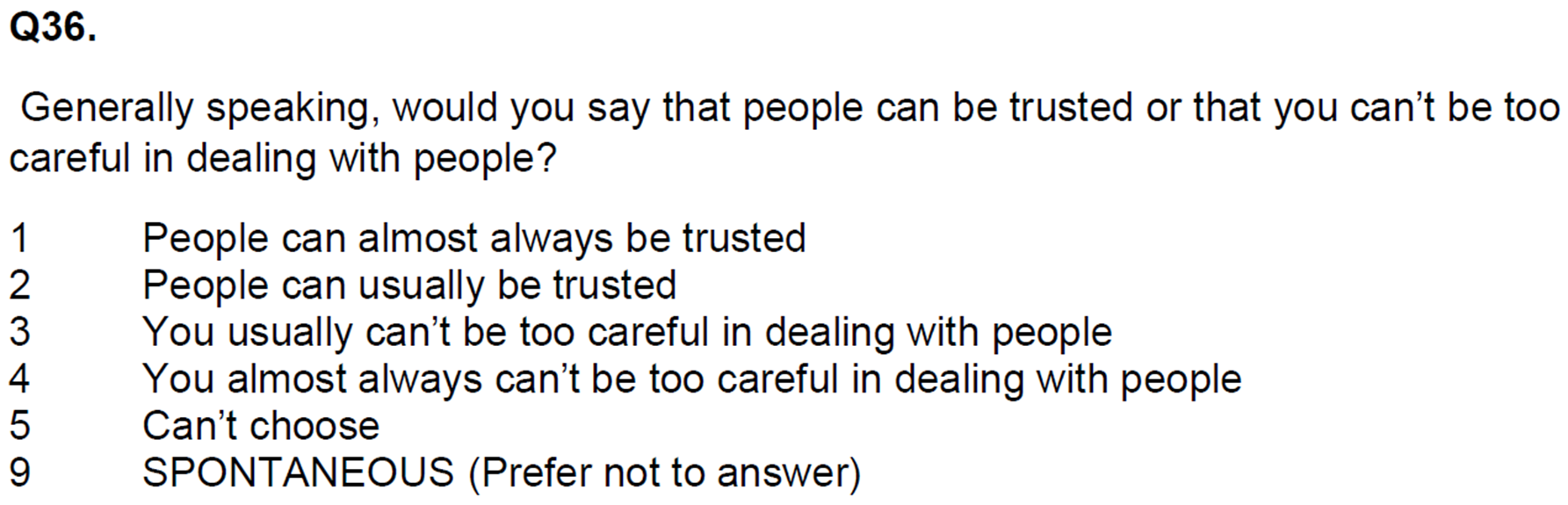
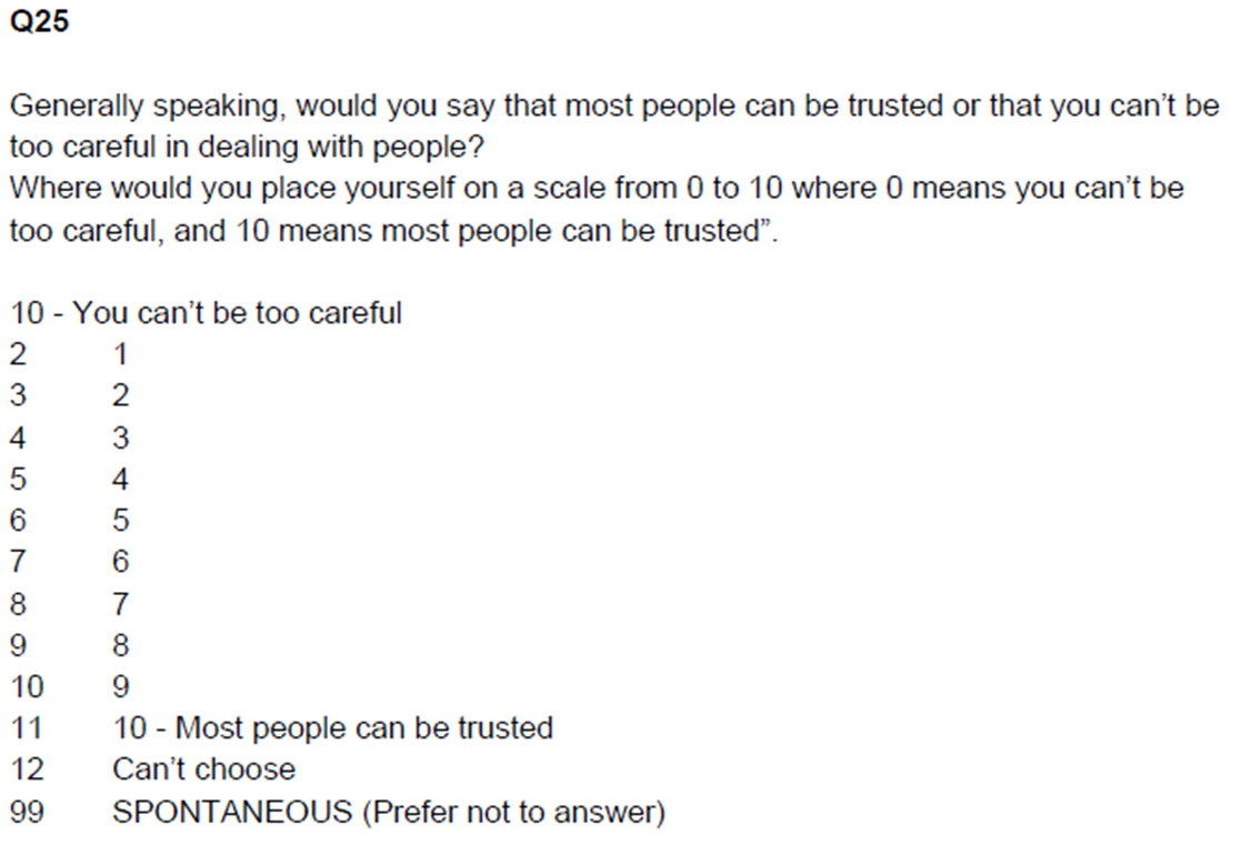
If you recall from Workshop 1, where we explored the different ways in which the concept of “social trust” is commonly operationalised in social surveys, the question was asked in two different ways in the 2010 BSA precisely with the purpose of testing their strengths and weaknesses. Figure 1 shows how the questions were asked in two different versions of the questionnaire. The gb-bsa10-trust dataset includes both versions.
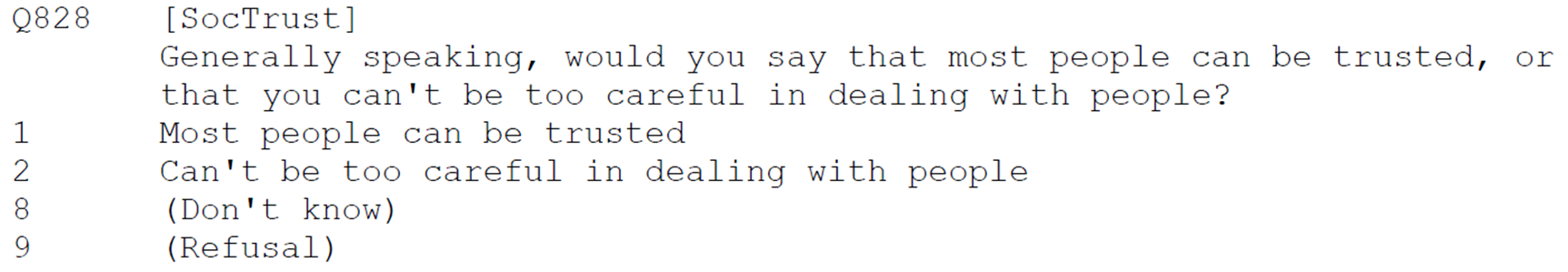
SocTrust)
PeopTrs3)
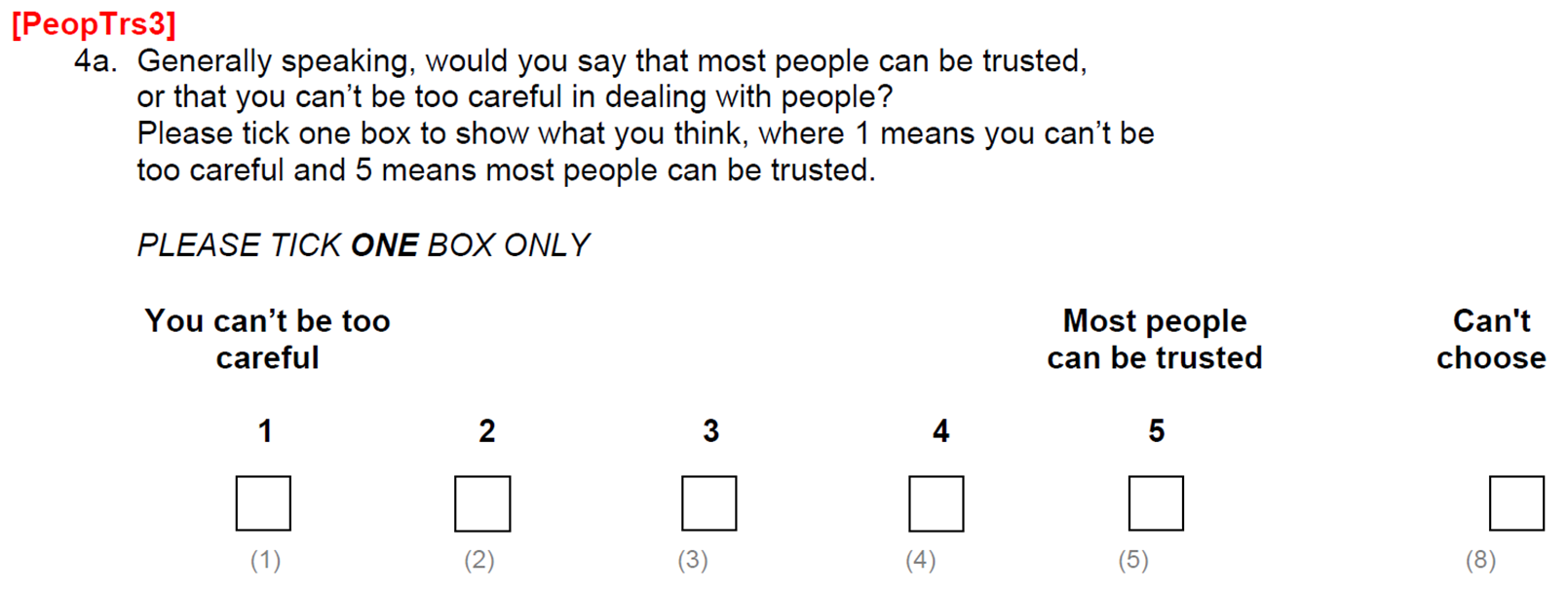
It may be worth noting that the survey participants did not answer both questions. The full BSA participant pool was divided into three groups and each was administered a different version of the questionnaire. In our dataset, the ABCVer variable tells us which of the three versions (A, B or C) each responded completed. Requesting Descriptives Statistics for the two “social trust” variables \(Split\) by the ABCVer variable, we can check which question respondents to each version have answered and how many responses they each produced (Figure 2).
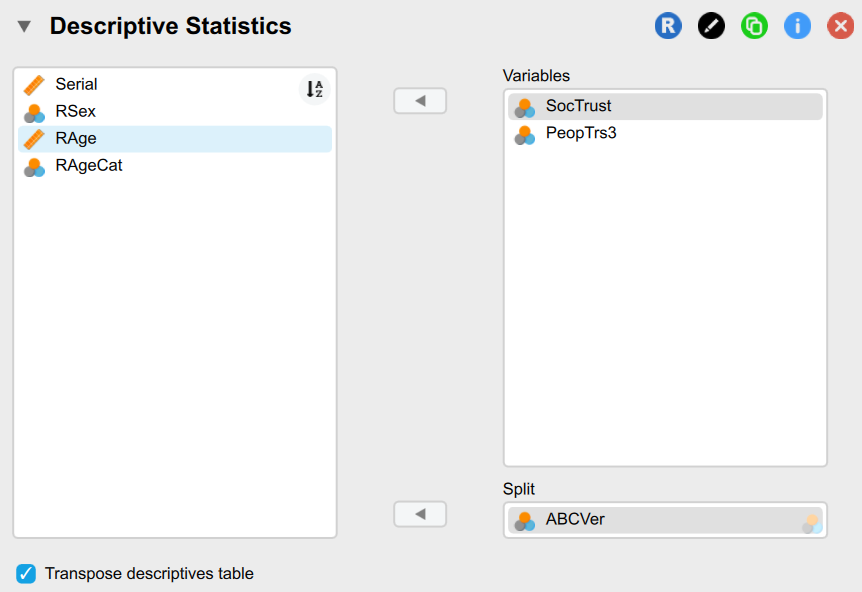
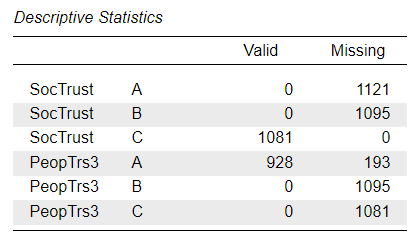
We can also see from the output that those answering version B of the questionnaire (n = 1,095) were not asked either of the “social trust” questions, so we should expect a high level of missingness by design in the dataset, which is not a problem because such missing values have happened “at random”, due to randomised allocation of respondents to one of the questionnaire versions. The real issue with high levels of missing data is when they are “missing not at random” (MNAR), but due to some underlying cause that can invalidate our measurement (e.g. very rich or very poor people may not be comfortable answering questions about their income, so they are more likely to choose a “prefer not to say” answer option).
Modelling SocTrust
We will first explore the variable SocTrust resulting from the Main Questionnaire version. As we can see from the questionnaire item in Figure 1 (a), this is the standard dichotomous “social/generalised trust” question which is also used in the WVS/EVS (the one from which the national-level “social trust” variables we focused on in the last two workshops were calculated as a national-level aggregate proportion of the number of those who had indicated that for them “most people can be trusted”). We are therefore expecting SocTrust to be a dichotomous variable in the dataset, although the “Don’t know” (8) and “Refusal” (9) answer options may not be coded as “missing” values, so we may need to perform some manual cleansing of the variable before we can use it in a regression.
Task 1: Summarise the variables
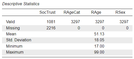
Task 2: Univariate descriptive analysis
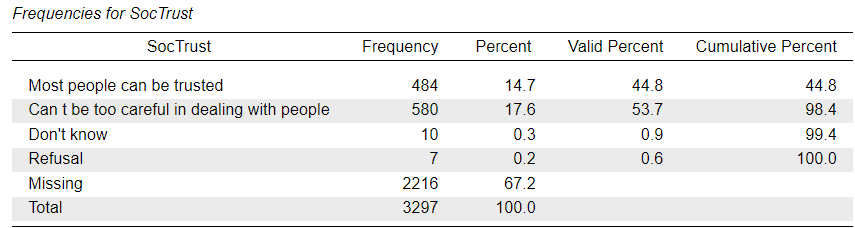
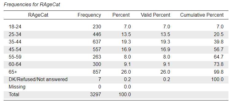
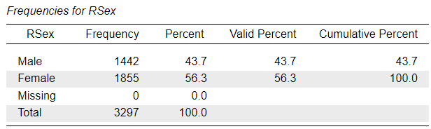
As we can see from the frequency distribution of the SocTrust variable, there is a very small number of responses in the “Don’t know” and “Refusal” categories, but these are treated as valid responses and not part of the “Missing” cases. The same is true for the RAgeCat variable - which is a version of the RAge variable with the ages collapsed into seven age-group “bins” - where the “DK/Refused/Not answered” category codes invalid answer options that are not considered as “Missing”. The RSex variable does not contain any such values.
Task 3: Data transformations
To address the research question, the SocTrust variable will serve as our outcome of interest, and we see that it is a categorical variable with two conceptually valid categories, so we will need to model it using binary logistic regression. The steps for fitting a logistic regression are very similar to those for a linear regression: Analyses Menu > Regression > Logistic Regression, which opens up an Analysis Panel that looks just like to one for linear regression (the options in the drop-down tabs will be different):


However, if we tried to enter the variable into the model in its original format, we would get an error message:
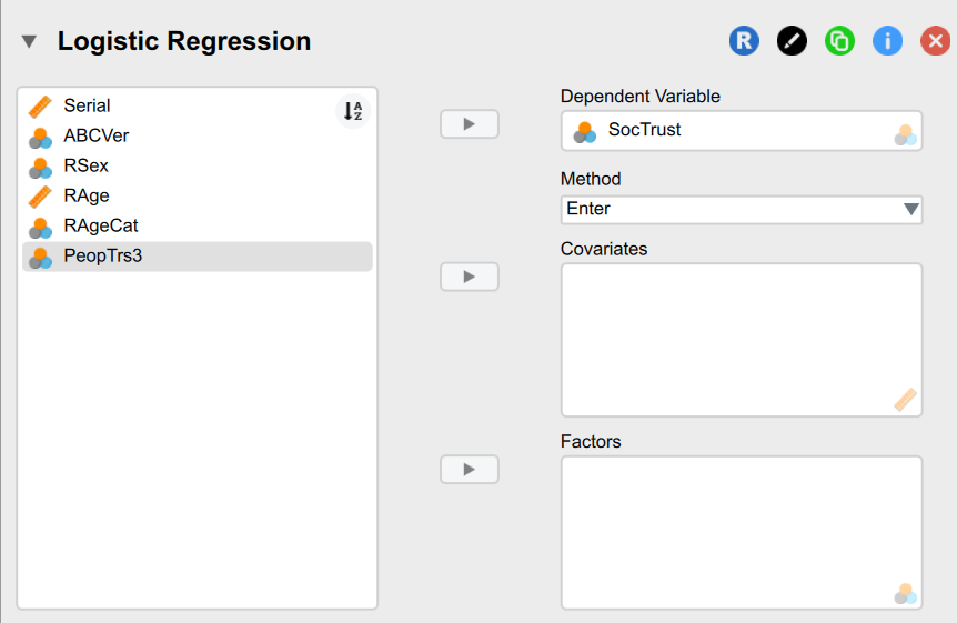
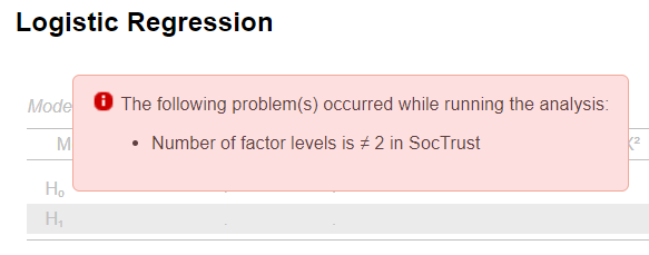
This tells us that currently the variable contains more than two valid category levels, and that’s because the “Don’t know” and “Refusal” categories are treated as valid. We will need to either remove them or reassign them as missing.
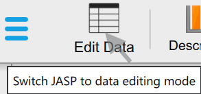
Filtering data and setting custom missing values
To manipulate variables, we will need to switch to the data editing mode:
In the data editor window, we can double-click on the column name we want to recode - in this case SocTrust. That will open up the “Label editor”:
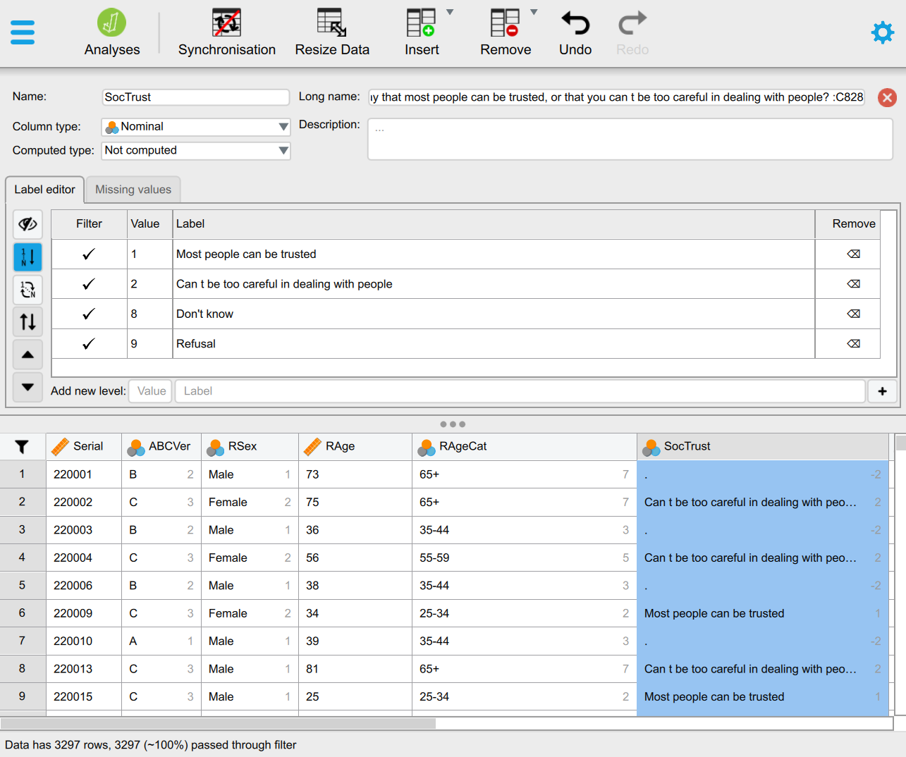
In the Label editor we have two main options for removing categories from the list of valid factor levels: (1) is to filter them out by un-ticking the appropriate tick-marks in the Filter column (see Figure 4 (a)) , or (2) by switching to the Missing values tab and entering the Values that we want to add to the list of custom missing values (see Figure 4 (b)). The result of option (1) is that the rows (cases/respondents) containing values on the SocTrsut variable that were filtered out will now be shown in light grey and will be excluded from statistical analyses (see Figure 4 (a)). This can be useful if we want to filter (or subset) the dataset for any reason, not just for the purpose of hiding invalid categories. We can easily un-filter the excluded values by ticking them again. The result of option (2) is that the additionally set custom missing values will be removed from the list of valid Values altogether. This is the technically correct solution for setting values as “Missing”. We can easily remove values from the custom missing list (see Figure 4 (d)).


Now do the same for the RAgeCat variable.
Having removed the invalid category levels from our dependent variable, we can check again the logistic regression model output. We should get the outputs shown in Figure 5. We see that now SocTrust is recognised as a dichotomous variable with only two valid categories, but the output Note highlighted in red is worth thinking about a little. It says that the “Can t be too careful in dealing with people” category, which we know from Figure 4 that it has the associated value “2” in the dataset, has now been automatically re-coded “as class 1”. What does this mean?

You should remember from the Section 1.2 that binary logistic regression assumes a binary/dichotomous/“indicator” type dependent variable that indicates the presence (typically coded as 1) or absence (coded as 0) of a specific qualitative characteristic, in our case “social trust”. And maybe you will also remember from the Workshop 3 Solutions Worksheet that JASP will automatically recode categorical variables entered into regression models into a series of indicator variables, one for each category/level measuring whether the case/respondent is part of that category or not (i.e. yes/no; 1/0; true/false).
What happened, then, is that JASP (as most other statistical software packages) automatically re-codes the dependent binary variable by giving its first category level the value “0” and the second level the value “1”. In our case, the second level was the one referring to the response option “Can’t be too careful in dealing with people” . So, we now have an outcome “scale” with only two values (0 and 1), with the category coded as 1 effectively indicating “mistrust”.
This is not technically a problem, but it may make the interpretation more awkward, so unless the concept we are specifically interested in is “mistrust”, it may be a good idea to change the ordering of the factor levels (categories), so that the category describing “trust” gets coded as 1 and the category describing “lack of trust” gets coded as 0.
Reverse ordering value labels
To reorder the values of variables in JASP, we return to the Label editor. The button to “Reverse order of all labels” is the one with the parallel up/down arrows; however, before we can use it, it may be telling us to first de-activate the “Automatic ordering of labels by their values” (the button highlighted in blue) (Figure 6 (a)). Once we click on that button to deactivate it, we can reverse the order of the labels (Figure 6 (b)).


As we can see in the data table, this doesn’t change the data, but it is already enough for the logistic regression fitting to change the ordering of the values in the dependent variable, and if we look at the regression outputs, we see that something has indeed changed:

Manually re-coding values
While simply reversing the ordering of the value labels may be enough in this case, it may be useful to manually recode the values to 0 and 1, so that we have a consistent treatment of the SocTrust variable across different analyses. If we don’t we may end up confusing ourselves later. We can go back to the Label editor and we can click in the cell containing the value we want to change. In this case, we can keep the value 1 as it is, but we can change the “2” to “0”, as in Figure 7 below:


We can also see in the data spreadsheet that this time the values themselves have changed in the dataset. When we save our dataset, we should keep in mind that we now have an altered dataset.
The logistic regression output won’t change a bit as a consequence of this manual re-coding, because we have just done by hand what the fitting function would have done for us automatically.
However, if we were performing a different type of analysis - for example a linear regression, which does not automatically apply any changes to the scale of the outcome variable - we would be noticing differences (compare the two versions of the outputs from a linear regression model for SocTrust before and after re-coding it to a “dummy”/indicator/(0/1) coded variable).

SocTrust M0, original coding of 1/2
SocTrust M0, after re-coding to 0/1Question
- You already know how to interpret linear regression results, so think about the two outputs above: what is the
(Intercept)in each version telling us, and why is there a difference? - If you’re struggling to answer, the Workshop 3 Solutions Worksheet will help (but leave it for later)
Manually editing labels
Before we continue with the data analysis - because we are in the Label editor anyway - we may want to perform a few additional “cosmetic” changes. All the fields in the Label editor can be manually modified, so we could change the variable names, value labels, long names, column types for any variable (just click on the header showing the variable/column name in the data spreadsheet below the Label editor. For example, we can prettify the names of the variables will will use for the analysis so that the labels in the outputs are clearer. In the examples below, I have changed the variable names of RSex, RAge, RAgeCat and PeopTrs3, and I corrected the missing apostrophe in the “Can t be too careful in dealing with people” label in SocTrust:


We can now continue with the analysis.
Task 4: Bivariate descriptive analysis
Task 5: Simple regression model
We have already seem in Figure 3 how to start a binary logistic regression analysis, and if you have followed along, then you should already have an output for a null model (M0), now updated with all the changes you have done to the data. You should be seeing something like in Figure 10 :

Currently the output only shows the “null model” that contains no explanatory variables. As in the case of the M0 in linear regression models, it only tells us the Intercept value. However, unlike in linear regression, the (Intercept) coefficient cannot be directly interpreted as the grand mean value on the original scale of the dependent variable, because because a dichotomous “scale” cannot really have an “average” value: one either is included in a category or not. How then do we interpret the Intercept coefficient (and more generally logistic regression coefficients)?
Proportions, probabilities, odds and logits
It may be useful to recall the Descriptive statistics at this point, particularly the Frequency distribution of SocTrust:

We know from the frequency distribution that there are fewer respondents in the sample who “trust” compared to those who “distrust”, by around 9 percentage points. So the M0 coefficient we see in the logistic regression output seems to quantify this difference in a different way. But how?
The frequency distribution also tells us that the proportion of “trust” in the sample is \(0.454\) \(\left(45.4\% = \frac{45.4}{100}\right)\) and that of “mistrust” is \(0.546\). Proportions are by nature measured on a \(0-1\) scale, where \(0\) is \(0\%\), \(0.5\) is \(50\%\) and \(1\) is \(100\%\), so any numeric value between the two extremes has a meaning. Proportions can thus also be thought of as “probabilities”, as “probability” is another statistical concept that is measured on the \(0-1\) scale. We could say, for example, that if we were to randomly draw individual rows (respondents) from our total sample of 1,060 respondents who had valid answers on SocTrust, we have a \(0.454\) probability of drawing someone who answered that “Most people can be trusted”. This is our best estimate given that we don’t yet know anything else about the characteristics of the sample other than the overall frequency distribution of SocTrust. Now this description is very similar to the one we gave to the Intercept in a linear regression “null model”: the mean value (average) of SocTrust is our best and safest prediction for the value of any individual observation of SocTrust given that we don’t (yet) know anything else about the data (i.e. other variables).
In fact, remember the output from the linear regression of SocTrust from earlier in Figure 8 ?
Indeed, when entering the SocTrust into a linear regression model after re-coding its values to \(0/1\) , the linear regression coefficient on the Intercept tell us precisely that the expected “mean” value of the SocTrust “scale”, which the model must assume to be an unbounded numeric scale on which we just happened to only observe two values (0 and 1), but where other values should be theoretically possible. If the size of two categories is not extremely “unbalanced” (e.g. a poll asking you whether you are enjoying statistics right now would likely result in a highly unbalanced response, with almost all the responses concentrated in the “No” (0) category), then even with this obviously mistaken assumption linear regression can give us acceptable estimates, as in this case. In fact, linear regression is so often used as an easy shorthand method for modelling dichotomous outcomes that it has a fancy name: linear probability model.
As mentioned in the Section 1.2, logistic regression attempts to overcome the limitations of the mistaken assumptions made by linear regression whilst retaining its logic of linearity. It does so by transforming the binary/dichotomous scale to an artificial one that resembles a continuous numeric scale, with countable values in between the 0 and the 1. As we saw earlier, the probability scale is such a scale and it is inherently related to proportions which can be used to characterise the relationship between the two categories of a dichotomy. So, logistic regression wants to relate predictors (like age or sex) to a probability, but ordinary straight-line (linear) maths can give numbers below 0 or above 1 — which don’t make sense as probabilities. One artificial scale that we can use to overcome this issue is the “logistic” or “logit” scale - that’s where the name of the regression method comes from. The logit is a clever re‑coding that turns a probability (0–1) into a number that can be any real value (−∞ to +∞). That lets us use a straight line on that transformed scale, then turn it back into a probability.
There are three “simple” steps for calculating a logit and converting between probabilities, odds and logits:
- For example, we have a probability p = 0.4537736, which is a very precise version of the proportion of “trusting” in our dataset \(\left(\frac{481}{1060}=0.4537736\right)\).
- Convert probability to odds: \[\mathrm{odds} = \dfrac{p}{1-p}\] For \(p = 0.45\ldots\) this is: \[\dfrac{0.45\ldots}{0.54\ldots} \approx 0.8307427\]
- Take the natural logarithm of the odds (this is the logit): \[\operatorname{logit}(p) = \ln\!\left(\dfrac{p}{1-p}\right)\] For odds \(\approx 0.8307427\), this is: \[\operatorname{logit}(p) = \ln(0.8307427) \approx -0.1854346.\]
Now if we compare the result from the manual calculation above to the (Intercept) coefficient estimate in M0, we find that these values coincide. In other words, the logistic regression is telling us exactly the same thing as the linear regression model, just on a strange artificial scale: the \(-0.185\) logit value is a slightly more accurate equivalent of the \(0.455\) probability value given by the linear regression model.
From the above equations we can also see that if the proportion/probability that we are modelling would be precisely \(0.5\) (i.e. \(50\%\), “trust” and “distrust” would have exactly the same number of responses), then the \(odds\) would be equal to \(\frac{0.5}{0.5}=1\) , and \(logit(p)=ln(1)=0\) . In other words, a logit value of \(0\) equals a probability value of \(0.5\), meaning equal probability. So, a negative “Estimate” coefficient in logistic regression has the same interpretation as a negative “Unstandardized” coefficient had in linear regression: a one-unit increase in the value of the predictor variable is associated with a decrease in the expected value of the dependent variable. It’s only the scale of measurement that is different to interpret.
The “Odds Ratio”
Since the logit scale is very abstract and difficult to decode, the most that we can get out from it directly is the sign (does it show an estimated increase or a decrease?). To be able to interpret the substantive meaning of the model in more detail, it is worth transforming the coefficients back into more easily understandable scales of measurement. One such re-conversion is to odds, which is also displayed in the logistic regression output table as the “Odds Ratio”.
In the manual calculations above, this was an intermediate value: \(\mathrm{odds}_{trust} \;=\; \frac{0.45\ldots}{0.54\ldots} \;\approx\; 0.830\ldots\)
The odds “scale” is one that is more familiar to the gamblers among us, but it’s often used in the interpretation of logistic regression results because it can be interpreted in percentage terms (although it is more involved when interpreting negative coefficients, as in this case). It is worth noting that the value 1 on the odds scale is equal to the 0.5 of the probability scale and the 0 of the logit scale: it signifies complete equality (no difference or change between the two values). Anything lower than 1, then, represents a decrease, and anything higher than 1 an increase. As expected, our value of \(0.831\) (rounded up) is lower than 1, so it shows a decrease. But by how much?
If the odds of our outcome are \(0.831\), that means that the odds are about \(16.9\%\) lower than “even odds” (\(1.00\)): \((0.831 − 1) × 100\% = −16.9\%\) (i.e. odds decrease by \(16.9\%\) per unit).
We can therefore say that a randomly selected observation (respondent) from our dataset has \(16.9\%\) lower odds to be in the “trusting” category.
This is a common way of interpreting coefficients from the logistic regression model, but it also has the drawback that when we report our results we may forget that the percentages of change we report are on the odds ratio scale, which is itself not a very self-evident one to most normal people. It is therefore better to re-convert the logit or odds value to the probability scale, which is simpler to understand because it runs from \(0-1\) and has that connection with proportions and percentage distributions that most of us are more familiar with. Even better, in JASP we can very easily request a visualisation of the coefficients in terms of probability. That will make more of a sense once we start adding explanatory variables to our model.
We now know all the statistical concepts, components and calculations that allow us to interpret logistic regression coefficients. So far we still only have a “null model” (M0), but interpreting the coefficients of explanatory variables should now be relatively straightforward, as it follows the logic we have learnt from linear regression applied to the logit-transformed scale we learnt above:
the
Interceptgives us a baseline expectation for the dependent variable - either its mean (in linear regression) or the logit-transformed probability/proportion of the indicator (“1”) outcome category (in logistic regression) - and the predictor coefficients move that baseline in either a positive or negative direction to give a better estimate of the outcome given what we can learn from the included explanatory/predictor variable(s).
We fit our simple logistic regression of SocTrust on Age and we should be getting something like this:


Logistic regression output: M1 with a single predictor (Age)
We should be able to interpret the results as saying:
- the effect of
Ageis positive but small, each additional year of age being associated with a \(0.006\) higher expectedSocTrustscore on the “log-odds” scale, or equivalently, with a \(0.6\%\) higher odds of being “trusting”. In other words, older people may be ever so slightly more “trusting” than younger people, but if so, only by a tiny amount (and furthermore, our estimates may not even be all that reliable - but more on this in Workshop 5 on Uncertainty and Inference). - Just as in liner regression, the
(Intercept)is now telling us the predictedSocTrustvalue of someone aged “0”. As we know, thisInterceptis now losing it’s substantive meaning, so unless we centre or standardise our numeric/“Scale” predictor variables, we should not worry about attempting to interpret theIntercept- it’s in the model only to provide a mathematical baseline for the other coefficients. - We won’t focus on the statistics shown in the Model Summary, but it’s enough to know that the columns shown (“McFadden R2”, “Nagelkerke R2”, etc.) are all different attempts to provide a simple estimate of the strength of the model as a whole, as the R2 value did in the case of linear regression, and they are interpreted roughly in the same way, telling us how much of the unexplained variance in
SocialTrustthe model (with all the explanatory variables taken together) helps explain. Each of the statistics has been highly debated in the statistical literature because the mechanics of logistic regression make it more difficult to calculate accurately such a generic value, but all of them taken together can give us an inkling of the explanatory strength of the model. In our case, since we only have a single predictor, these values are close to the actual coefficient value forAge, and tell us that the model is indeed not very strong.
Task 6: Multiple regression model
You should now have all the information needed to fit and interpret a multiple logistic regression model that can give us an estimate of how “age” is associated with “social trust” in a British population in 2010-2011, when adjusting for “sex”.
One useful reporting trick - especially when we also have categorical/indicator predictors - is to plot the coefficients on a probability scale. If you recall, this means that we re-convert the “log-odds” and the “odds ratio” coefficients to probabilities, which has some nice properties - it runs from \(0-1\), just like proportions - allowing for easier interpretations.
We can do that by requesting [Inferential plots >] Conditional estimates plots under the plots drop-down option set, which will result in the following output:


Logistic regression: Conditional estimates plots
Modelling PeopTrs3
To model this variable, we need to recode the values of PeopTrs3 manually so it only has 0 and 1 values. That means that we need to make a decision on how to group together the individual values of the \(1\ldots5\) valid scale on which the variable was measured. We could recode all values from \(1-3\) into \(0\) and \(4-5\) into \(1\), or could have \(1-2\) as \(0\) and \(3-5\) as \(1\). Run some univariate descriptive statistics and some bivariate visualisations to check the empirical distribution of the variable; think about the logic underpinning the variable and survey question; then you can make a decision that you can defend.
In practical data analysis you will often encounter situations when you will want to recode categorical variables into fewer categories than the original scale. Such a situation may emerge in the course of an assignment task in which the variable chosen as dependent variable in a planned regression model is multi-categorical (multinomial). There are special statistical models for such dependent variables, however, in this module we are not covering these more advanced methods. Instead, you will want to transform the variables - if logically, conceptually or theoretically possible - into binary/binomial/dichotomous variables (i.e. variables with only two categories).
Such transformations are easy to implement in JASP, and the procedure amounts to manually re-coding the values of the categories by giving several categories the same values. I demonstrate how to recode multinomial variables in the two videos below:
To follow the example transformations in the demo videos, you can use the data_transformation dataset available to download from the module website’s Data page.
Task 1: Summarise the variables
Task 2: Univariate descriptive analysis
Task 3: Data transformations
Task 4: Bivariate descriptive analysis
Task 5: Simple regression model
Task 6: Multiple regression model
Task 7: Interpretation
Exercise 4.1.2. Citizenship Survey, 2010-2011

Task 1: Summarise the variables
Task 2: Univariate descriptive analysis
Task 3: Data transformations
Task 4: Bivariate descriptive analysis
Task 5: Simple regression model
Task 6: Multiple regression model
Task 7: Interpretation
Exercise 4.2: Do young people (under-24s) have lower social trust in post-pandemic Britain?
You will use the following three datasets, in turn, to model social phenomena in “post-pandemic” Britain:
- Community Life Survey 2023-24 (
gb-cls23-trust_nm.sav) - British Social Attitudes Survey 2024 (
gb-bsa24-trust.sav) - British Social Attitudes Survey 2023 (
gb-bsa23-trust.sav)
Exercise 4.2.1. Community Life Survey, 2023-2024
Read the research question carefully and identify what it does and doesn’t tell you about the variables, data selection and modelling methods that are needed to address the question as directly as possible. Consider the following questions in particular:
- Which “age” variable would you choose if you had more than one option available, and what kind of transformation may be useful in order to answer your research question?
- Do you need to transform your outcome/dependent variable, or can it be modelled as it is? (You may have different option here!)
- If you wanted to fit a binary logistic regression model, how would you need to transform the outcome variable, if at all?
- Can you fit two different types of regression models and compare the results?
- Do you have any other eligible “control” variables at your disposal in the dataset? If so, what would be the benefit of including them in the model?
Task 1: Summarise the variables
Task 2: Univariate descriptive analysis
Task 3: Data transformations
Task 4: Bivariate descriptive analysis
Task 5: Simple regression model
Task 6: Multiple regression model
Task 7: Interpretation
Exercise 4.2.2. British Social Attitudes Survey, 2023
The “social trust” variable in this dataset poses similar (but somewhat simpler) data transformation challenges to those encountered with the 2010 BSA (Self-completion) “social trust” variable.
Task 1: Summarise the variables
Task 2: Univariate descriptive analysis
Task 3: Data transformations
Task 4: Bivariate descriptive analysis
Task 5: Simple regression model
Task 6: Multiple regression model
Task 7: Interpretation
Exercise 4.2.3. British Social Attitudes Survey, 2024
The “social trust” variable in this dataset is similar to the one encountered in the 2023-2024 Community Life Survey.
Task 1: Summarise the variables
Task 2: Univariate descriptive analysis
Task 3: Data transformations
Task 4: Bivariate descriptive analysis
Task 5: Simple regression model
Task 6: Multiple regression model
Task 7: Interpretation
Exercise 4.3: Which of the assignment research questions could be addressed using a logistic regression model?
Let’s look again at the assignment research questions. Some of these questions imply a dependent variable which is measured as a numeric scale or at least a long-ish (e.g. 7-point +) ordinal scale in one of the surveys we will use for the assignment (ESS10, WVS7, EVS2017). Other questions imply dependent variables that are more strictly categorical, and as such, we cannot model them using linear regression. For those, we may be able to apply a logistic regression model.
If your chosen outcome variable is categorical with more than two categories but fewer than at least seven, you will have to dichotomise it in order to use it as a dependent variable in a logistic regression. While there are specific modelling methods for “multinomial” type outcome variables, we are not covering them on this module.
In this exercise, explore the assignment dataset using the Variable search function on the website to identify any available variables for answering one/some of the questions below, and check how the implied dependent variable was measured:
- Are religious people more satisfied with life?
- Are older people more likely to see the death penalty as justifiable?
- What factors are associated with opinions about future European Union enlargement among Europeans?
- Is higher internet use associated with stronger anti-immigrant sentiments?
- How does victimisation relate to trust in the police?
- What factors are associated with belief in life after death?
- Are government/public sector employees more inclined to perceive higher levels of corruption than those working in the private sector?
JASP solutions
Below you can download JASP files with solutions to some of the exercises in this worksheet: