Workshop 3 Worksheet
Learning outcomes
By the end of the session, you should be familiar with:
- fitting and interpreting simple and multiple linear regression models in JASP
- the basic ideas behind variable standardisation
- the options and limitations of comparing the performance of linear regression models
- the differences in interpretation between numeric “Scale” and categorical “Nominal” predictor coefficients
Intro
The exercises in this worksheet will introduce linear regression, building up from simple bivariate (single-predictor) regression models to more complex ones that include a combination of numeric and categorical explanatory variables.
Exercise 3.1: How is income inequality associated with social trust?
We continue where we left off in the last Workshop, taking further Workshop 2 Worksheet - Exercise 3 in which we explored the relationship between income inequality by social trust visually through a scatter plot using data related to the analyses presented in Wilkinson and Pickett (2009) (Figure 4.1) and Pickett, Gauhar, and Wilkinson (2024) (Figure 7). For this, we used the pickett2009.csv and pickett&al2024.sav datasets, respectively, which are available for download from the Data page of this website.
In that exercise we focused mainly on the scatterplot in order to practice creating visual representations of bivariate associations. In this exercise, our focus will instead shift to understanding what the “regression line” is actually telling us, before we move on to expanding our analysis with additional explanatory variables.
Task 1: Visualise the relationship between social trust and income inequality
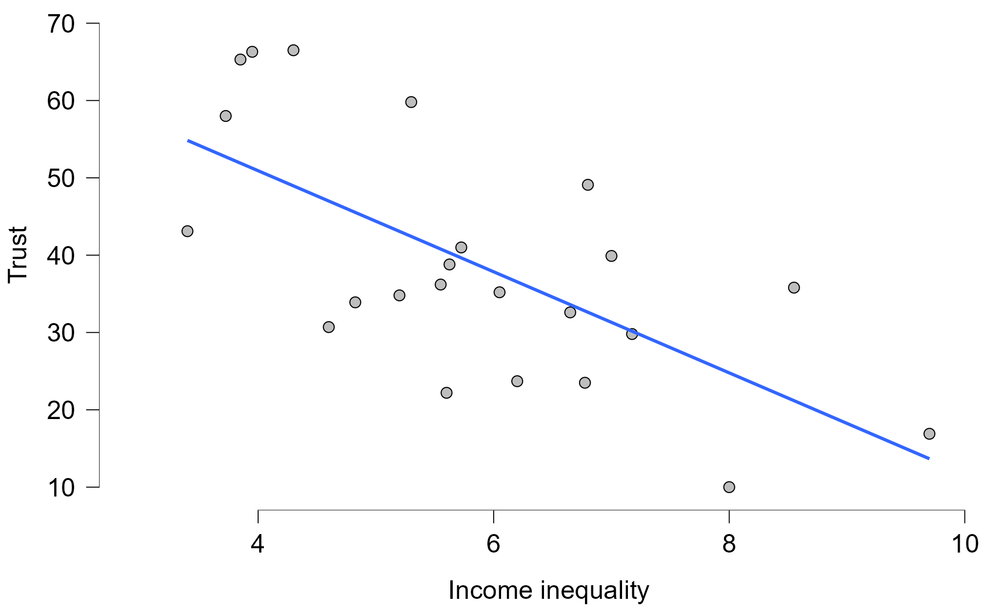
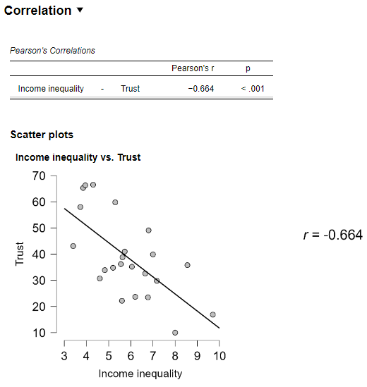
As a first step, create a scatter plot visualising the “relationship” between social trust (Trust) and income inequality (Income inequality) (read more about the measurement of income inequality here to better understand the meaning of this variable). This is Exercise 3 from Workshop 2.
A quick way to visualise the bivariate relationship between your chosen variables is by using the Descriptives > Descriptive Statistics [Customizable Plots] option set. There, depending on the combination of the types of variables you have, you can choose the most appropriate plot type. In this case, because we have two Scale type variables, the most appropriate plot type is a Scatter plot. You can use the various available settings to simplify your plot or make it more complex, as desired. For example, it is sometimes useful to simplify the scatter plot produced by default by removing the univariate density plots from the margins of the scatter plot and removing the grey shading of the confidence interval. All of these provide important additional information about the two variables and their relationship, but it can also make the plot too complex for a quick visualisation.
When done, you should be seeing something like this:
If you need a reminder of how to do it, check Workshop 2 Worksheet.
Task 2: Fit a simple (bi-variate) linear regression model
The scatter plot includes the [Add regression line] option by default because it represents a very useful visual summary of the relationship between two Scale type variables. However, it doesn’t provide any precise statistical description of the relationship: we can see that it is a “negative” association (i.e. the higher the level of income inequality the lower the level of Trust, but we cannot see precisely how strong that association is.
To dig deeper into the meaning of the regression line, we can fit a simple (bivariate) linear regression model of social trust as a function of societal inequality (i.e. a model aiming to explain/predict values of social trust in various countries depending on the value of income inequality in those countries).
To build a linear regression model in JASP, click through the Menu tabs:
\[ \text{Regression} \longrightarrow \text{[Classical] Linear regression} \] In the Linear regression panel, move the Trust variable to the \(\text{Dependent Variable}\) box and the Income inequality variable to the \(\text{Covariates}\) box. By doing this, we are essentially saying that we want to use the Income inequality variable to help predict the mean of the Trust variable (i.e. we treat Trust as the dependent variable, the one we wish to “explain”/“predict”/“model” as a linear function of our independent variable(s).
The results from the linear regression model will appear in the outputs window on the right. You should be seeing something like this:
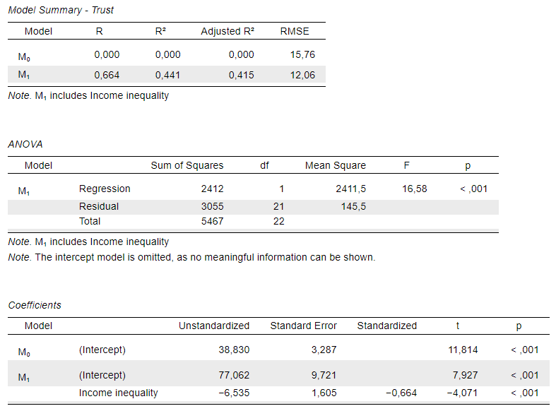
Interpret the regression model output
In general terms, the coefficient of interest (the one associated with the independent variable) tells us: that a one-unit difference/change on the independent variable scale is associated with a difference/change in the dependent variable of the size shown by the value of the coefficient.
But what does this mean substantively in the context of our two variables?
Questions
- Using the lecture slides and the essential readings for this week, interpret the meaning of the regression coefficient on
Income inequality. In the output, we are looking at the third table (Coefficients) under the Unstandardized column; - Add a note on the JASP output under the \(\text{Coefficients}\) output and write down your interpretation there. [Tip: You can add notes on your JASP outputs by hovering over the name of the output (e.g. the “Coefficients” table title and clicking on the small black down-arrow that appears next to the text, then clicking “Add Note” in the drop-down list) ]
- Where can you find the coefficient of correlation (\(R\)) in the outputs? What about the coefficient of determination (\(R^2\))? What do these tell you - how do you interpret them?
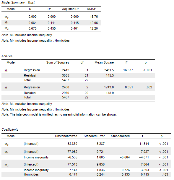
The Model Summary and the ANOVA tables describe a few overall model statistics. For our immediate purposes, however, these two tables are less useful. We can turn out attention more closely to the Coefficients output table, and within that we should first focus on the Unstandardized column, which lists the regression coefficients associated with our predictor variables.
What is the meaning of the regression coefficient on the (Intercept)?
The Coefficients table presents results from two “models”. One is a model without any explanatory (independent/predictor) variables (M0), in which case the (Intercept) is the only relevant value and is nothing more than the average (mean) value of the outcome (dependent/explained) variable calculated on the sample of cases/observations (i.e. countries here) that were included in the analysis (i.e. only those who had a valid measurement on both of the variables Trust and Income inequality). We are told that this average value is 38.8, and knowing that the Trust scale measures the percentage of people who are more trusting than not in each country, we can interpret this as 38.8%. This “null model” (M0) is given to us by default in JASP, without us asking for it.
The model we actually fit is presented as M1, and this is what we are interested in. As we see in the Coefficients table, the coefficient associated with the (Intercept) value in M1 is no longer the mean/average level of Trust on its own (38.8), but instead 77.06. This value represents the expected score on the dependent variable (Trust) when the value of the independent variable (Income inequality) equals 0. As it will become apparent from the discussion below, a value of 0 for the Income inequality variable is highly unrealistic, and it is often the case that the Intercept does not tell us a meaningful value. However, that’s not a problem, because the (Intercept) value is meant to provide a mathematical baseline for the model and we generally are not interested in interpreting it. It’s enough to know what it means in principle. When we expand the analysis to a multiple regression, the meaning of the intercept will be even more complex and its interpretation is near impossible. If we want to get a meaningful value for the Intercept, we could centre or standardise our modelled variables.
A simple “centring” would involve shifting the scale such that the mean of the scale falls on the value 0, and any values below the mean become negative values. For example, if we were to “centre” the scale of numbers between 0 and 10, we would transform the following “scale”:
0 1 2 3 4 5 6 7 8 9 10
… into this one:
-5 -4 -3 -2 -1 0 1 2 3 4 5
The length of the scale is still the same (10 units), as is the difference between the units (4-3 = (-1) - (-2) = 1); but now the mean value is 0 instead of 5.
Then, the Intercept could be interpreted as the expected value of the dependent variable when the value of the independent variable is at its mean. However, this then makes it less straightforward to interpret the regression coefficient associated with out predictor variable on the original scales on which the variables were measured. And what we really are interested in is the coefficient on our independent (explanatory/predictor) variable.
What is the meaning of the regression coefficient on Income inequality?
In general terms, the coefficient of interest (the one associated with the independent variable) tells us that a one-unit difference/change on the independent variable scale is associated with a difference/change in the dependent variable of the size shown by the value of the coefficient.
But what does this mean substantively in the context of our two variables?
We see that the regression coefficient associated with our predictor/independent variable is -6.535. This tells us that a one-unit increase on the Income inequality scale is associated with a -6.535-units change on the Trust scale. To give this a more meaningful interpretation, we need to know what exactly a “unit” and a “one-unit change” means on each scale, and for that we need to remind ourselves what our variables actually measure.
What is a “unit”?
Understanding the measurement scale of the Trust variable is straightforward. We know that it measures the percentage of respondents in each country who answered that “in general, most people can be trusted” to the standard social trust survey question in the World Values Survey. That means that the theoretical scale runs from 0(%) to 100(%). A unit on this scale is therefore one percentage point. The coefficient of -6.535, then, means a reduction of 6.5% (rounded to one decimal point) in the national aggregate level of social trust.
Understanding the Income inequality scale is trickier. It denotes the so-called “income quintile share ratio”, a commonly employed measurement of inequality in a country’s income distribution. It is calculated as the ratio of total income received by the 20% of the population with the highest income (the top quintile) to that received by the 20% of the population with the lowest income (the bottom quintile).1 For example, if in Portugal earners in the bottom quintile of the income distribution held 5% of the total income distributed in that country, while those in the top quintile of the distribution received 40% of that total. If we divide the two (\(\frac{40}{5}\)) we obtain 8, which is the Income inequality value we find for Portugal in the dataset.
This means that the minimum value that the scale can take is 1 (because \(\frac{10}{10}\) = \(\frac{40}{40}\) = \(\frac{50}{50}\) = \(1\) ), which would describe a perfectly equal society where the richest 20% of the population receives the same amount of total income as the poorest 20%. The maximum value, however, is theoretically infinite (because the measurement is a ratio, and e.g. \(\frac{90}{1}\) = 90, but \(\frac{99.9}{0.03}\) = 3330 and \(\frac{99.999}{0.00005}\) =1.99998^{6}), and the higher the value the more unequal a society is, with the total income of the poorest 20% of the population tending to 0. In reality, however, no society has ever achieved either of these extremes. The ratio is used to measure and compare real-world income inequality, where values typically fall on a much narrower empirical scale somewhere between these two theoretical limits. In our dataset, we know from the Descriptive statistics that the actual measured minimum value is 3.4 and the maximum is 9.7, so nowhere near the theoretical limits of the scale. You can read more about the measurement of income inequality in the dataset’s Codebook.
So, then, what does a one-unit difference/change mean?
It means, for example, the difference between an inequality score of 8 (e.g. Portugal) and one of 7 (e.g. Australia), or between a 5.59 (e.g France) and a 4.59 (e.g. Belgium). Therefore, our simple linear regression model predicts that a country whose Income inequality score is 7 (e.g. Australia) should have an associated Trust score that is 6.5 percentage points higher than that of another country whose Income inequality is 8 (e.g. Portugal). Given that we already know the Intercept (i.e. the predicted value of Trust when Income inequality is 0), we can get even more specific: the predicted Trust score of a country whose Income inequality is 8 (e.g. Portugal) would be: \(77.06 \text{ (Intercept)} + 8 \text{ (number of one-unit differences/changes from 0)} \times -6.5 \text{ (rate of change/slope/regression coefficient)}\) = 24.782; then, the predicted Trust score for a country whose Income inequality is one unit lower (i.e. 7), would be 24.782 - (-6.5) = 31.317.
More generally, however, we can say that our simple linear regression model predicts that a country with an inequality score 1 points higher than that of another country will have, on average, a trust score that is 6.5 units lower than that of the other country’s.
This prediction is far from perfect, as we can see from comparing these predicted values to the actual values observed in our data set (for example, Portugal’s measured Trust is not 24.7% but 10%, while Australia’s aggregate Trust level is 39.9%, not 31.3% as predicted). However, overall it is still a better prediction than we could have made had we not had any information about Income inequality. In that case, our best prediction could have only been the mean value of Trust on its own, which we know from the (Intercept) of the “null model” (M0) to be 38.8. This may be a somewhat more accurate prediction in the case of Australia, but it’s a much worse one for Portugal and most of the other countries in the dataset. Ultimately, even this simple linear regression model helps us make a better informed assessment of the variability in social trust across countries, even if it will either overestimate or underestimate any given individual value.
Furthermore, as we will discuss later (see Workshop 5 on Uncertainty and Inference), our real aim when conducting such an analysis is to generalise beyond our empirical sample (our dataset) to the more abstract theoretical “population” that our sample is meant to represent. The information provided in the columns Standard Error, t and p will be useful in this respect, as they allow us to assess the confidence we can have in the generalisability of our model given the level of uncertainty inherent in our data.
There are further complications with the substantive interpretation of a “one-unit change” on the Income inequality scale, which we will not be considering here, but they are worth noting.
We interpret a value of 8 (e.g. Portugal) to mean that the top quintile in that country earns eight times more than the bottom quintile, and a value of 5.59 (e.g France) to mean that the top earns ~five and a half times more than the bottom.
However, given that its unit of measurement is a “ratio”, the “income quintile share ratio” is fundamentally a measure of multiplicative difference, and so it is non-linear: the relative impact (or percentage increase in inequality) associated with a one-unit change in the ratio is not consistent across the entire scale, but it decreases as the ratio gets larger. For example:
- a ratio change of 1 to 2 represents a relative increase in inequality of 100% (doubles), which is a massive relative change;
- a ratio change of 4 to 5 represents a relative increase in inequality of 25% (a quarter), which is still a significant relative change;
- a ratio change of 20 to 21 represents a relative increase in inequality of 5%, which is a much smaller relative change.
This means that moving from a ratio of 7 (e.g. Australia) to an 8 (e.g. Portugal) represents a different relative increase in the income gap compared to moving from a ratio of 4.59 (e.g. Belgium) to 5.59 (e.g France), namely a difference of 14.3% and 21.8%, respectively.
For mathematical and statistical purposes, particularly when researchers need to compare changes in inequality across different populations or over time, a non-linear scale like the S80/S20 can be problematic. To handle this non-linearity, researchers often use a logarithmic transformation of the ratio in their models, which effectively linearises the scale and makes the interpretation of coefficients consistent across the entire range of values. Income inequality measured as the “income quintile share ratio” is not the only variable that is non-linear and would benefit from a statistical transformation. In fact, if we look at our dataset (pickett2009) we find a variable called Imprisonment (log), which - as it’s name suggests - has already been “log-transformed”.
As noted, this is not something that we will be worrying or thinking about in this module.
What is the meaning of the “Standardized” regression coefficient on Income inequality?
First of all, we should notice that apart from its sign (\(-\)), the number is the same as that shown in the R column in the Model Summary table. That’s no coincidence, because the “Standardized” coefficient for Income inequality is nothing else than the coefficient of correlation (\(R\)).
*What is the “coefficient of correlation*****” (\(R\))?
The coefficient of correlation (\(R\)) is calculated by standardising the scales of the two variables included in the regression model (Trust and Income inequality) and expressing the regression coefficient on that artificial standardised scale.
But what exactly does “standardisation” mean?
It simply means that we can mathematically alter the values of a scale so that the scale is redefined in some artificial unit of measurement which becomes directly comparable to other scales regardless of the differences in the units of measurement of the original scales, while keeping the relationship between the values equal to that of the original scale. One form of standardisation, which is most useful when we have categorical “scales”, is expressing observations as percentages instead of absolute values. Another commonly employed form of standardisation, which is more useful for numeric scales, is the so-called z-score, which tells us how many “standard deviations” (SD) each score/value is from the mean/average score/value on a given measurement scale. In fact, when you hear or read about a “standardised” scale, it is almost always this z-score standardisation that the author is referring to.
The \(z\)-score for an observed value \(x\) that is part of a scale of values \(X\) is calculated as: \({(x-\overline{X})\over{s_X}}\), where \(x\) is any single value on the \(X\) scale, \(\overline{X}\) is the mean of \(X\) and \(s_X\) is the sample (observed) standard deviation of \(X\). Expressed in words: we subtract the average of the \(X\) scale from each individual value \(x\) and then we divide that number by the sample standard deviation of the \(X\) scale. You can read more about how the sample standard deviation itself is calculated here
So, then, how do we interpret the “Standardized” regression coefficient?
On these newly standardised scales, a value of 1 should be interpreted as “one standard deviation above the mean”, a value of 2 means “two standard deviations above the mean”, a value of -1 means “one standard deviation below the mean”, and so on. This means that the two standardised variables are measured on a similar scale and their values are therefore directly comparable, which was not the case for the original unstandardised values.
In JASP, we can use the zScores() drag-and-drop function to calculate this. If we were to create two new variables that are the z-standardised versions of the Trust and Income inequality variables, respectively, and we ran the same regression as above on those variables, then the obtained regression coefficient on “standardised income inequality” would have coincided with the correlation coefficient and it would have been -0.664.
A coefficient of -0.664 associated with “standardised income inequality” would therefore be interpreted as: a one-standard-deviation positive change in “income inequality” is associated with a roughly two-thirds of a standard deviation (around 66.4%) negative change in “social trust”.
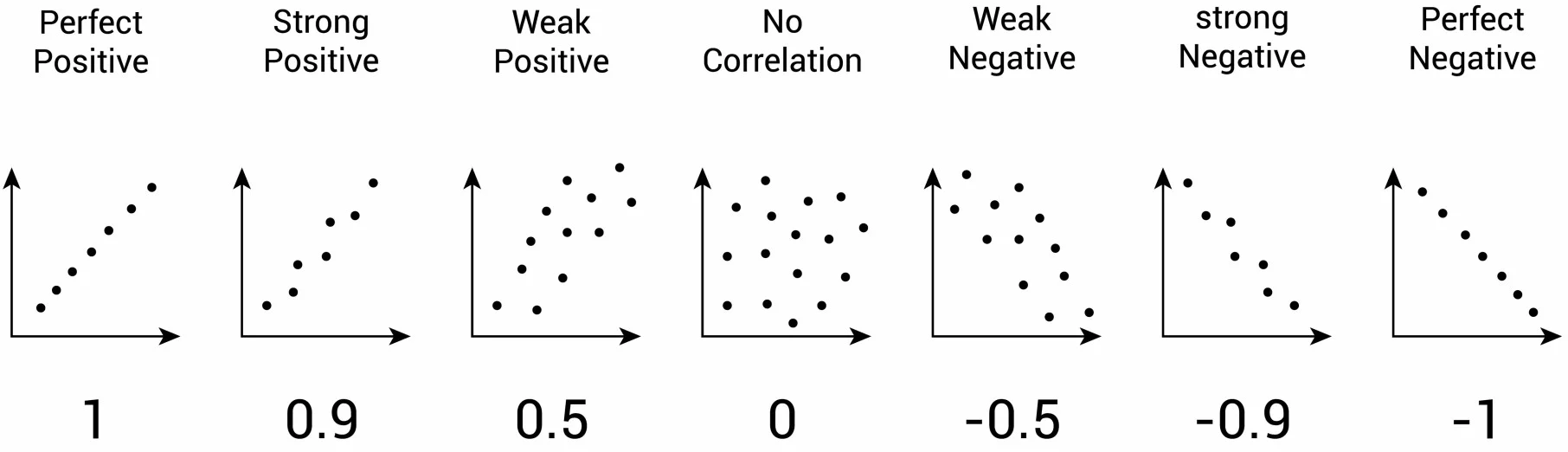
However, the purpose of the “correlation coefficient” is to provide a more general description of the association between two numeric variables. Its value ranges between -1 and 1, where 1 represents a perfect positive correlation between the two variables and -1 a perfect negative correlation, while 0 shows no correlation between the two at all. Visualising some of these extreme and intermediate correlations on scatter plots would look something like this:
What about the coefficient of determination (\(R^2\))?
As its notation suggestes (\(R^2\)), the coefficient of determination is simply the squared values of the coefficient of correlation (\(R\)). We can find it in the Model Summary output table in the column labelled R2. We find that this value is \(0.441\), and if you want you can check manually whether this is really the square of the \(R\) value, \((-0.664)^2\).
The coefficient of determination can be a very useful summary statistic for the entire mode, especially if we have a more complex multiple regression model. It summarises how much of the variance in Trust can be explained overall by the explanatory variables included in the model, taken together. It is a very useful summary because it can be interpreted on a percentage scale, so we can say something like: our regression model - which only includes Income inequality - can help explain \(44.1\%\) of the variability in Trust.
Task 3: Find the correlation coefficient using a “correlation” test instead
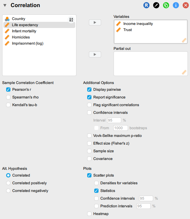
To run a simple correlation analysis in JASP, go through the Menu tabs:
Regression > {Classical} Correlation
Move both of the variables of interest to the \(\text{Variables}\) box.
In the settings, you can also choose to display a scatter plot by ticking the option [Plots > Scatter plots] and you can also tick [Plots > Statistics] to display the correlation coefficient to the right of the scatter plot. You should be seeing something like this:
Check if the results align with those obtained using linear regression in the previous task. The results should look something like this:
As we can see, we can obtain the same statistics from the linear regression model, and regression modelling is a more versatile tool, so we can use it instead of the Correlation option.
One thing that is particularly useful in using regression modelling is that we can extend the model to incorporate the effect of more than one independent/explanatory variable. We will look at this in the next exercise.
Exercise 3.2: How is income inequality associated with social trust when we also adjust for the potential influence of homicide rates on social trust?
As mentioned earlier, the coefficient estimates we obtained from the simple linear regression in Exercise 3.1 are probably not the “best”. We have attempted to explain the variation in Trust only as a function of Income inequality, whereas there may be other social factors that can influence the average levels of social trust in a society. In fact, it may even be the case that one of these other potential factors that we have not considered is itself associated with income inequality to a degree that makes it a much better predictor of social trust. If we can hypothesise - based on existing literature or common sense - that there are other factors at play and we can measure them, we could try to adjust for their potential influence on social trust and get a “better” - or “clearer” - estimate of the true association between income inequality and social trust. For example, what if the difference in the rate of homicides in a country is what makes people trust each other less or more? It could be a plausible assumption that people may have less trust in strangers if they hear about cases of homicide more often and perceive their environment as more dangerous. It may even turn out that countries with higher homicide rates happen to have higher levels of income inequality, but it is in fact the homicide rate that is the stronger predictor of social trust.
What are homicide rates?
Homicide rates usually measure the number of homicides per 100,000 residents. It is calculated by dividing the number of homicides recorded in a country in a given year by the total population and multiplying the result by 100,000. E.g. if there were 600 homicides in a population of 1,000,000, you would divide 600 by 1,000,000, then multiply the result by 100,000: (600/1,000,000) x 100,000 = 60 per 100,000.
In our dataset we do have a variable Homicides that measures national-level homicide rates, so we can use it to test the above assumptions. We can simply add that variable to our model as a second explanatory variable, turning our model into a multiple linear regression (i.e. a regression model with one outcome (dependent) variable and more than one explanatory (“independent”, “predictor”) variable).
Task 1: Assess the association between Homicides and Trust
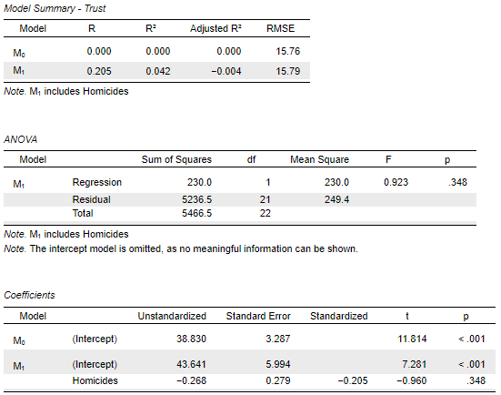
Although for our research question we are primarily interested in understanding the association between Income inequality and Trust, to be able to compare different outputs and build up our understanding of how linear regression works in practice, we can start by fitting another simple linear regression, this time regressing Trust on Homicides to check the association between them. Performing this step no longer requires detailed guidance, but once done you should be seeing something like this output in the results panel:
Questions
- Using the lecture slides and the essential readings for this week, interpret the meaning of the regression coefficients in this output. You can add a note on the JASP output under the \(\text{Coefficients}\) output and write down your interpretation there.
- Can we directly compare the coefficient for
Homicidesto that we obtained forIncome inequalityin the earlier analysis? Can we say that one predictor is “stronger” or “more influential” than the other? If yes, which is the “stronger” predictor? If no, why not? - What does the coefficient of determination (\(R^2\)) tell us about this model? Can we say that one model is “stronger” or “better” than the other? If yes, which is the “stronger” model? If no, why not?
What is the meaning of the regression coefficient on the (Intercept)?
Our dependent variable is the same as in the previous exercise, and we know that the (Intercept) value is nothing more than the average (mean) value of the outcome (dependent/explained) variable calculated on the sample of cases/observations (i.e. countries here) that were included in the analysis (i.e. only those who had a valid measurement on both of the variables Trust and Homicides). Because Homicides and Income inequality have the same number of observations (there aren’t any observations/countries with missing values on either), the sub-sample used in this regression is the same as the one in the previous analysis. Therefore, the value of the (Intercept) in model M0 is also the same: 38.8. However, when we take the Intercept to mean the expected value of Trust when Homicides is equal to 0 (M1), we find that the (Intercept) value is 43.6, so for a country that has absolutely no homicides, we expect that 43.6% of the population would feel that “most people can be trusted”. Interesting…
Purely based on the Intercept, and compared to what the Intercept was in the previous regression analysis when we considered the influence of Income inequlity on Trust, would you say that the rate of Homicides is a strong(er) or weak(er) predictor of the level of Trust in a society?
What is the meaning of the regression coefficient on Homicides?
We see that the regression coefficient associated with our predictor/independent variable (Homicides) is \(-0.268\). This tells us that a one-unit increase in Homicides is associated with a \(0.268\)-unit decrease in Trust. For example, the Homicides value for Belgium is 13 and for the United Kingdom is 15 in the dataset, meaning that the difference between the two countries is two units. Based on our simple linear regression model, therefore, we would predict that the United Kingdom’s Trust value should be \(0.536\) Trust-units (i.e. ~0.5%) lower than that of Belgium (because \(2 \times -0.268 = -0.536\). However, to reiterate, the main aim of the model is not necessarily to give us very accurate predictions of individual values, but to give us the most reasonable estimate of what we could expect to see in the wider “population” given the empirical data we have in our dataset.
Can we directly compare the coefficient for Homicides to that we obtained for Income inequality in the earlier analysis?
We know that in the earlier analysis the regression coefficient for Income inequality was \(-6.535\). Obviously, \(6.535\) is a larger number than \(0.268\) - so, can we say that Income inequality is associated with a much, much larger negative difference in Trust than are Homicides? To answer this, we again have to think carefully about the scales of our variables and the meaning of a “one-unit” change in the context of each scale of measurement.
We have already established that Income inequality refers to the “income quintile share ratio”, so its scale can run from a minimum of 1 (perfect equality) to theoretical infinity (extreme inequality), although the empirical scale that we actually observe in our dataset runs from 3.4 to 9.7. This means that the scale contains just over six units, each measuring one ratio. The Homicides scale, on the other hand, runs from 5.2 to 64 (check the Descriptive statistics!), so we have almost 60 units. That’s a much “longer” scale, on which a single unit means 1 homicide for 100,000 people in the country’s population. Can we say and expect that a difference between 7 and 8 homicides per 100,000 people should have a comparable effect on Trust to the difference between an income quintile share ratio of 7 and an 8? This is similar to expecting that a body weight unit of 1 (kg) should have the same influence in an adult’s Body Mass Index (BMI) calculation as that of 1 unit of height (cm), even though there are fewer units (kg.) of weight (85 for the male average) in a human body than there are units (cm) of height (176 for the male average).
Due to such differences in the scales that are being compared, it is very common to “standardise” the variables used in a regression so that each unit involved is “equal”. On the other hand, the difficulty is then shifted onto interpreting those standardised coefficients on the original meaningful scale of the variables involved. In other words, it’s a challenge either way. In this exercise, we have left the two variables involved in the regression unstandardised, so a “unit” has a different meaning in the case of each variable, and we should keep this in mind when interpreting their effects. They are not directly comparable unless we choose to standardise their scales.
What does the coefficient of determination (\(R^2\)) tell us about this model? Can we say that one model is “stronger” or “better” than the other?
We already know from before that the \(R^2\) value is literally the square of the \(R\) value, and we also know that the \(R\) value is a standardised coefficient, so \(R^2\) is also a standardised measure, meaning that it is directly comparable to other \(R^2\) values, unlike the individual regression coefficients. This, then, means that we can compare the \(R^2\) values of the different models to assess which one is “stronger” or “better” at explaining the unexplained variance in our dependant variable.
In the Model Summary output table, in the column labelled R2 , we find that this value is \(0.042\). In other words, our regression model - which only includes Homicides - can help explain only \(4.2\%\) of the variability in Trust. Compare this to the\(44.1\%\)explanatory value of our previous model - which only included Income inequality - and we can fairly state that the Homicides model is “weaker” or “worse” at explaining the variability observed in the Trust variable.
Task 2: Fit a multiple linear regression model
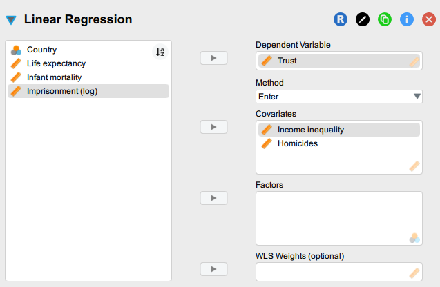
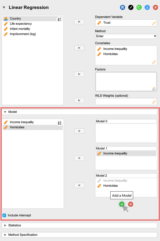
In JASP, if our independent variables are of Scale type, we add them into the Covariates box - just as we did with Income inequality - and if they are categorical (Nominal or short Ordinal) variables, then we add them to the Factors. In the latter case, JASP will automatically recode the categorical variables into a series of “dummy” (i.e. binary, dichotomous) variables, one for each category/level measuring whether the case/respondent is part of that category or not (i.e. yes/no; 1/0; true/false). In our current dataset (pickett2009.csv), all of the variables that can logically serve as predictor variables are measured on a Scale level, so we will move them to the Covariates. If you add the Homicides variable to the Covariates, the input panel (left) should look something like this:
The output in the results panel (right) should show something like this:
We can simply continue the Linear regression analysis we started in Exercise 3.1, or we can start a new Linear Regression analysis in the same JASP workbook. If we start a new Linear Regression, we have the advantage of then being able to see both sets of outputs in the results panel.
JASP also allows us to build up several different “nested” models as part of a single analysis, which then has several additional benefits: all the models will be summarised in the same output tables (e.g. as M0, M1, M2, M3, etc.), providing additional statistical comparisons across all the fitted models, ensuring that the same sub-sample is used across all models even if the dataset is “unbalanced” in the sense that some of the explanatory variables have more missing values than others.
To achieve that, we first (1) need to move all the explanatory variables that we want to include in our most complex model into the Covariates or Factors boxes (in our case we move Income inequality and Homicides), then we can (2) roll down the Model drop-down tab and click on the green \(+\) sign to add another model (e.g. Model 2). This new model will include all the variables included in the previous model (e.g. Model 1), allowing us to include some further variables. First, we should simplify the previous model (e.g. Model 1) by removing some explanatory variables (e.g. Homicides) from it (moving them into the box on the left); this frees the variable up so that it can be included in the next model (e.g. Model 2) instead. With our example analysis, the Model options tab in the input pane (left) should end up looking something like this:
And the output in the results panel (right) should show something like this:
We see that the output combines the results from our earlier simple linear regression model and from our new multiple regression model. In this case the values are exactly the same regardless of our approach, but if one of our explanatory variables would contain missing observations, then the sub-sample of the data used in each model would differ if they were fitted independently from one another (i.e. not “nested” as here), which would in turn affect the estimated coefficients.
Remember: we should make our choice of predictor variables based on theoretical and conceptual grounds, while also ensuring that the statistical criteria for the choices are also met. You know from the Essential Readings (see. Goss-Sampson 2025:75) that linear regression makes a number of “assumptions” about our data and variables:
- Outliers: there should be no significant outliers, high-leverage or highly influential data points;
- Linearity: there should be a linear relationship between (a) the dependent variable and each of your independent variables, and (b) the dependent variable and the independent variables collectively;
- Independence: the observations should be independent from one another (i.e., independence of residuals; e.g. no repeated observations from the same participants/cases, as in a longitudinal analysis that would ask the same question of the same person at different points in time);
- Normality: the model residuals (errors) are approximately normally distributed;
- Homoscedasticity: the variance of residuals (errors) are approximately equal;
- Low multicollinearity: avoid including two or more independent variables that are highly correlated with each other.
Of these, the potential for high levels of “collinearity” or “multicollinearity” (i.e. when the predictors themselves show a high level of dependence on each other) may be something to consider in the case of our data, as the variables we have available in the dataset should - in theory at least - be correlated with each other to some significant degree. This can be an issue because it inflates the variance of the coefficients, making them less reliable.
To get a sense of how much of an issue this is for our analyses, we can inspect the correlation between the predictor (“independent”, “explanatory”) variables themselves. It is worth noting that multicollinearity emerges as an issue when core explanatory variables of interest are highly correlated with each other after accounting for all the other variables included in the model. In other words, if we have more than two explanatory variables that may be collinear in a model, we must ensure that
The coefficient of correlation between the predictors will tell us how strongly the predictors are correlated, and if we were to subtract that correlation coefficient from 1 and then divide 1 by the result of that subtraction \(\left(1 \over {1 - R^2}\right)\), we would get a commonly used statistic for assessing multicollinearity called the Variance Inflation Factor (VIF). In JASP, we can request this statistic directly under the Statistics drop-down tab by ticking the [Tolerance and VIF] option. Read more about the VIF and when multicollinearity is (not) a problem in this short blog entry
We now have a statistical model which explains variation in Trust as not only dependent on Income inequality, but also on the rate of Homicides. Put differently - if our main aim is to estimate how Income inequality is associated with Trust - we have obtained a more accurate estimate of the association between Income inequality and Trust, because we have additionally also account for variation due to differences in the homicide rates in each country, which in itself can have an impact on how much trust people have in strangers.
Another way in which this “account for” is often expressed is that the stated coefficients are those obtained after we adjust for or keep constant or eliminate or control for the effect of the other variable(s) in the model - although often this terminology is highly confusing as it seems to imply causal relationships (“effect of…”) and experimental interventions (“keep constant…”, “control…”), which is not something that linear regression analysis can achieve on its own when using survey data. So: beware of causal and experimental design language when you encountering it in your readings, and try to avoid it as much as possible in your own writing!
This procedure is expected to give us more accurate estimates because by including further (but carefully selected on conceptual grounds!) variables into the model, we have removed them from the pool of the “unknown” factors affecting/related to our outcome variable of interest.
Questions
- Using the lecture slides and the essential readings for this week, interpret the results.
- How has the association between
Income inequalityandTrustchanged once we have adjusted for the potential influence of theHomicidesrate in a country? - Based on this model, what is the expected difference in the average level of measured
Trustif we observe a one-unit higher level in the rate of homicides? - What is the coefficient of determination (\(R^2\)) telling us now? Is our multiple regression model “stronger” or “better” than our earlier simple regression models?
The interpretation of the coefficients is similar to the one we gave in the simple linear regressions earlier, with one important adjustment: now each coefficient tells us the expected difference in the value of Trust associated with a one-unit change in the given predictor while the values of all the other predictors in the model are kept constant (i.e. their effect is nullified, taken out of the equation, etc.).
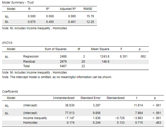
This means that the coefficient of \(-7.147\) for Income inequality is a more precise estimate of the impact of Income inequality on Trust than the coefficient obtained earlier from the simple regression model (\(-6.535\)) , because this coefficient now also accounts for the expected effect of the rate of Homicides in each country.
Vice-versa, we may actually be interested in the effect of Homicides itself on Trust, and the interpretation works in the same way: the model expects/predicts that each one-unit positive change in the rate of Homicides will be associated with a positive (the is no negative sign!) change of \(0.174\) units on the Trust scale, whilst we also adjust for the variation in Income inequality across the countries.
Now this should be somewhat surprising to us given the result we had from the earlier single-predictor model. When we did not adjust for the effect of Income inequality, a one-unit increase in Homicides was associated with a predicted negative change (reduction) in Trust of \(-0.268\). So, not only did the coefficient in the multiple regression model become smaller (\(0.17\) vs. \(0.27\)), but it actually changed its sign ( \(+\) vs. \(-\) )! This tells us that Homicides is an unreliable predictor in this model and we should think carefully about whether this multiple regression model is “better” or “worse” than our simple regression model.
We have not yet considered closely the meaning of the other columns in the Coefficients table (we will in Workshop 5 on Uncertainty and Inference), but to make up our mind about what to do next we will also need to look at those columns. Without going into details about what it means, we see in the “Standard Error” column that the standard error associated with the coefficient on Income inequality is slightly larger (\(1.836\)) than it was in the simple regression model (\(1.605\)). This essentially means that the addition of Homicides has made the estimate of Income inequality more “error-prone”, decreasing the level of confidence we can have that it is generalisable to a wider population or phenomenon beyond our data.
What is the coefficient of determination (\(R^2\)) telling us now?
The correlation coefficient loses its original meaning in the context of a multiple regression model in which we have more than one predictor/independent/explanatory variable. It’s meaning becomes “partial” to all the other variables in the model. In this case, its squared value, the R2 is more meaningful. Looking at the R2 value we also find that this has increased slightly to 0.455, indicating that the combined knowledge of the Homicides rate and the Income inequality score of a country can help explain \(45.5\%\) of the variation in Trust. The remaining ~\(55\%\) of the variation is associated with other factors that our model is not (yet) adjusting for. If we have variables measuring factors that can potentially have a good explanatory value, we could consider them as additional Covariates/Factors to include in our models.
Is our multiple regression model “stronger” or “better” than our earlier simple regression models?
What is - or should be - interesting is that the multiple regression model appears “stronger” or “better” at explaining the variation in trust compared to the simpler model in which we only had knowledge of Income inequality (\(R^2 = 44.1\%\)) despite the fact that the additional Homicides variable itself turned out to be a very weak and unreliable predictor. This is often the case, because in principle any additional information that we can build into a statistical model should help reduce the amount of unexplained variance in the dependent variable. This is not always the case in more complex models, but in general it is a reasonable expectation. This is why it is useful to include a number of standard “control” variables - i.e. variables in whose coefficients we are not directly interested in, but we know from theory or previous experience that they can have an influence on sociological outcome/dependent variables. However, if we include many control variables that are weak and unreliable predictors without a good theoretical reason, we risk heightening the potential for multicollinearity in our models, potentially making the core explanatory variables of interest also less reliable.
In the case of out current regression model, there is no good reason for keeping Homicides in as a control variable in future models, given that it contributes very little to the explanatory potential of the model
Exercise 3.3: Multiple linear regression with categorical predictors
The purpose of this exercise is to demonstrate the interpretation of the effect of categorical explanatory (“independent”, “predictor”) variables included in regression models. In the pickett2009 dataset we do not have usable variables that could be treated as categorical, so for this exercise we will make use of another dataset. The delhey&newton2005 dataset contains variables that allow us to replicate - as closely as possible - parts of the analysis undertaken by Delhey and Newton (2005). The variables have been compiled from various sources based on the methodological details provided in Delhey and Newton (2005) and the slightly more detailed working paper version of the article.
The exercise consists of a number of tasks that allow you to practice the steps of quantitative analysis already learnt in previous workshops and exercises.
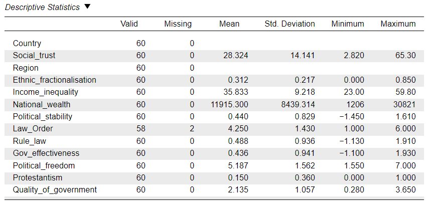
Task 1. Create a Descriptive Statistics table to summarise the distributions of all the variables in the dataset
When there are many variables in a dataset, it is often a good idea to “transpose” the Descriptive Statistics table so that variables are listed in the rows and the summary statistics in the columns.
When done, you should be seeing something like this:
Questions
- How many cases (i.e. countries) are in the dataset?
- What is the average level of “social trust” in the dataset as a whole (i.e. what is known as the “grand mean”)?
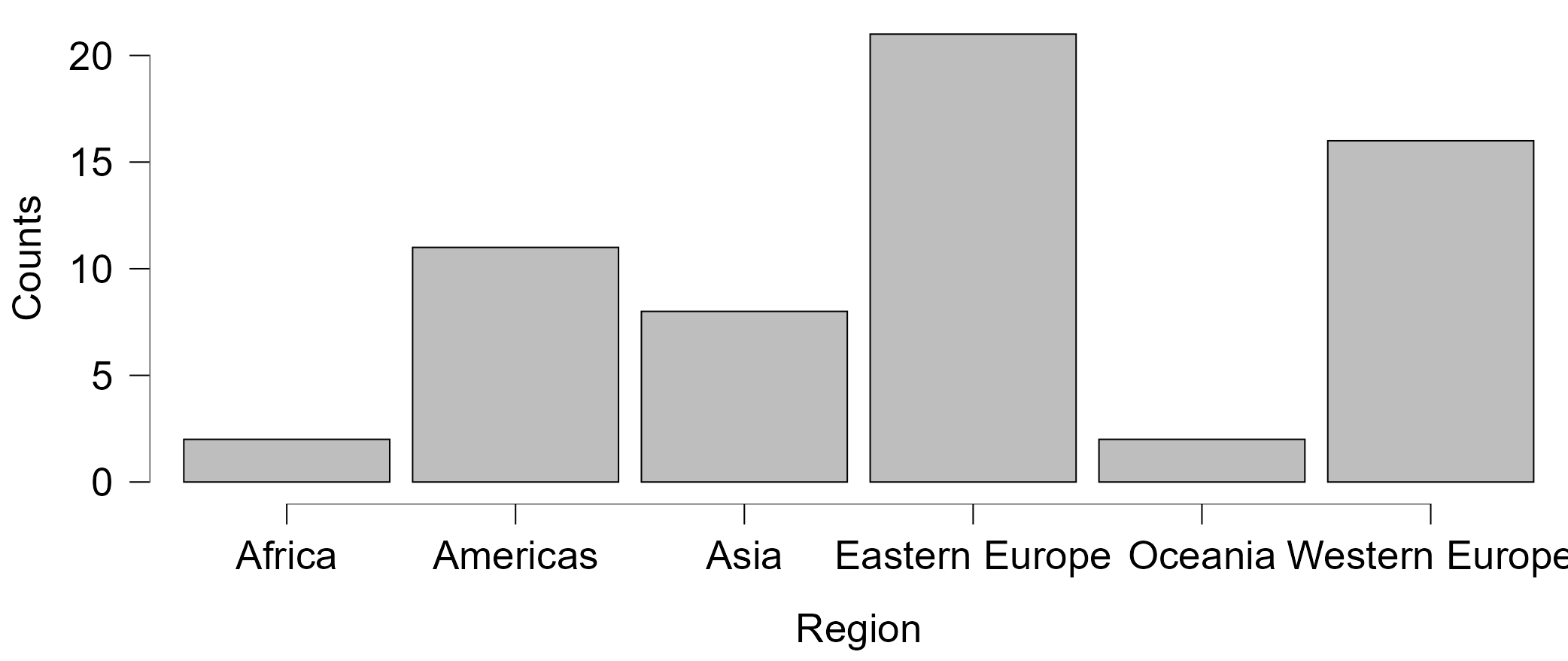
- Can we tell how many world Regions there are in the dataset?
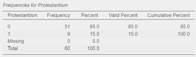
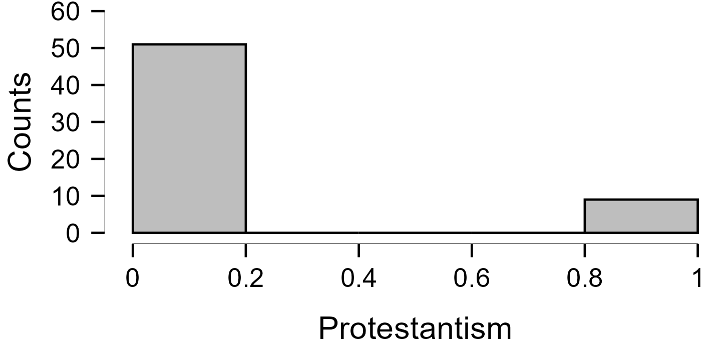
- What scale is “Protestantism” measured on? Can we tell how many categories the variable has?
Task 2: Identify any potential explanatory variables that can be treat as categorical variables and create the most appropriate univariate descriptive summaries
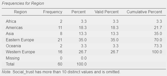
When done, you should be seeing some of these outputs:
Questions
- How many world Regions there are in the dataset?
- How is “Protestantism” measured? Is it a “scale” variable - as coded in the dataset - or a “Nominal” categorical variable? Does it make a difference?
Task 3: Create bivariate visualisations of the association between “Region”, “Protestantism” and “social trust”
When done, you should be seeing some of these outputs:
Questions
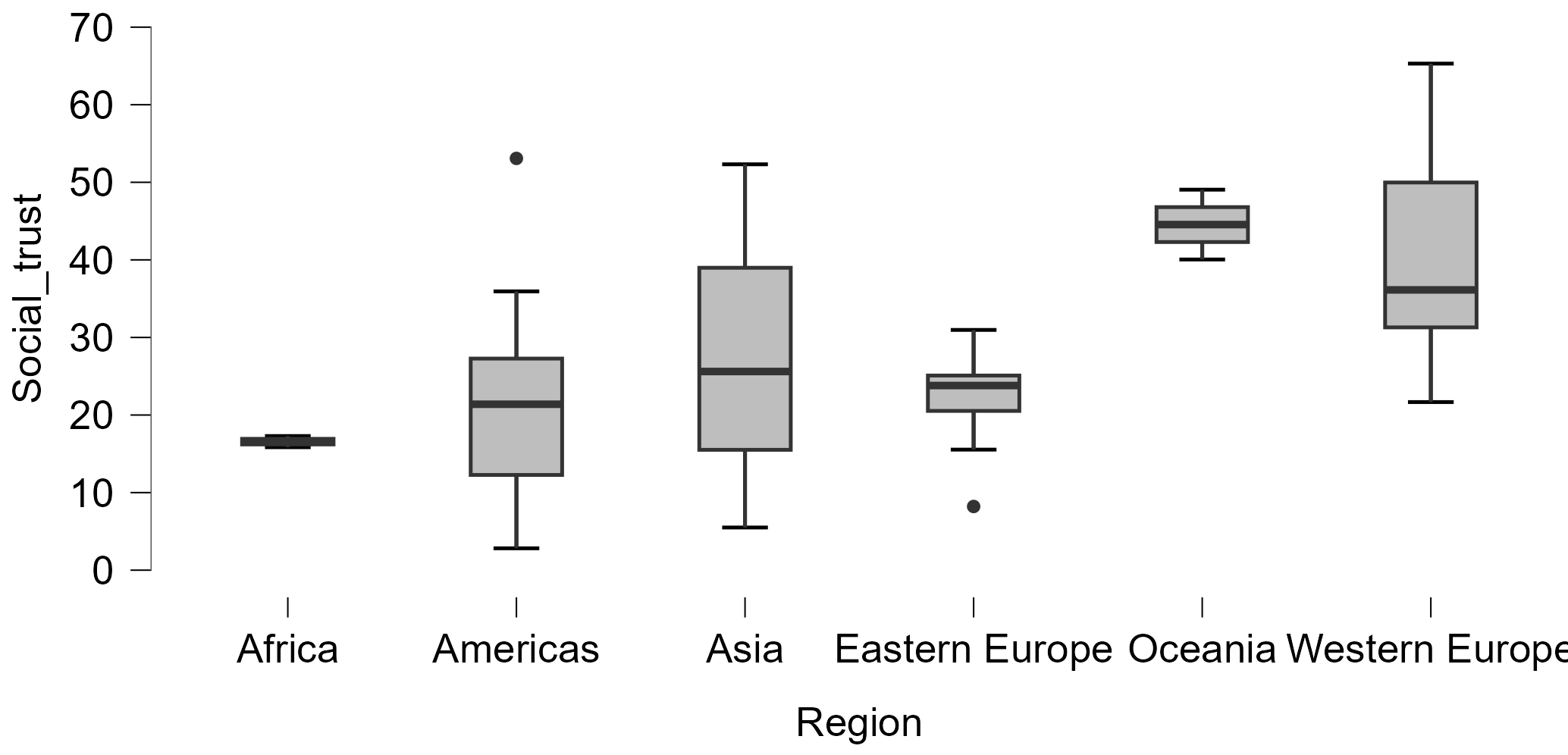
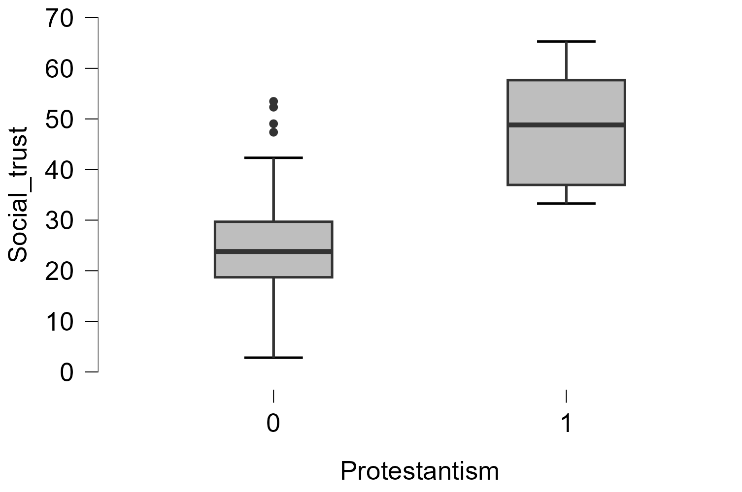
- Which “Region” has the highest and the lowest average level of “social trust”?
- Which “Region” shows the most and least variation in “social trust”? What may be the reason behind this variation?
- Are the Eastern European or the Western European countries more diverse in their levels of “social trust”?
- Which categories of “Region” and “Protestantism” show any outliers?
- Do Protestant or non-Protestant countries have a higher level of “social trust”?
Task 4: Fit a linear regression model to assess the relationship between “social trust” and the world “Region” of the country
Click through the Menu tabs:
\[ \text{Regression} \longrightarrow \text{[Classical] Linear regression} \]
In the Linear regression panel, move the Social_trust variable to the \(\text{Dependent Variable}\) box; but this time, we will move the Region variable to the \(\text{Factors}\) box instead.
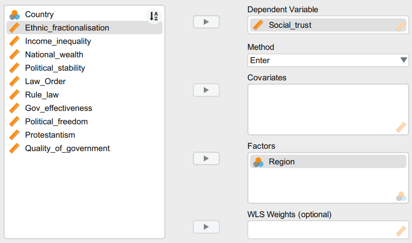
This will tell JASP that the Region variable is categorical and it should model it as such, treating each of its constituent categories as an individual factor/indicator variable.
When done, the outputs from the linear regression model will appear in the results panel on the right, and you should see some of these outputs:

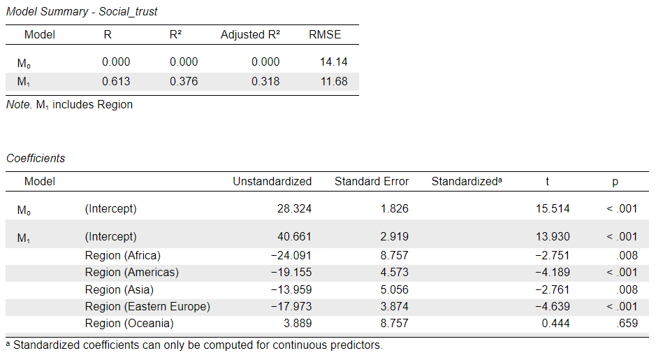
If we look carefully to the list of Regions in the Coefficients table, we notice that only 5 categories are listed, whereas we know from the descriptive statistics the there are six Regions in our dataset. What happens here is that JASP automaticallyleaves out the first category (Task 2 above will tell you which one that is) of “Factors” from the model so that the left-out category becomes the baseline/reference to which the coefficients on all the other categories compare. Essentially, the first category is given the value of 0 and each other category receives a value of 1 compared to the “reference category”; so, in the output the entry for “Region (Americas)” is essentially a dichotomous (binary, “dummy) variable in which”Americas” is coded as 1 and “Africa” (the left-out category) as 0; similarly, the entry for “Region (Asia)” compares “Asia” (1) to “Africa” (0) and “Region (Western Europe)” is a variable that compares “Western Europe” (1) to “Africa” (0).
What happens here is that the left-out category (here “Africa”) is absorbed into the Intercept (the unknown/unmeasured variation in the dependent variable), just like in the case of a numeric predictor the Intercept represents the predictor at value 0. Therefore, the regression coefficient for the (Intercept) represents the predicted Social_trust value for “Africa” (28.32% in M0 and 16.57% in M1 where the influence of other Regions is also accounted for). The intercept for “Region (Americas)” then tells us that compared to a country in “Africa”, a country located in the “Americas” is expected show a \(4.9\)-unit higher level of Social_trust. The biggest difference is that between “Oceania” and “Africa”, where countries in the former region are predicted to have a \(28\)-point higher Social_trust on average than those in “Africa”. And so on.
There are obvious problems emerging from the fact that some of the Regions have only few observations (countries), making the mean highly unreliable if not nearly meaningless. This is made even worse by the fact that the “reference” category to which all others compare is “Africa”, which has only 2 observations (countries) in the dataset despite being a continent consisting of 54 countries in reality (this makes it substantively different from “Oceania”, which is also only represented in the dataset with 2 countries - Australia and New Zealand - although these do cover a significant proportion of the population of Oceania in reality, which otherwise consists of 12 further countries that are mostly smaller island nations). A better option would be to choose a more stable/larger category to serve as the “reference”. This is not a difficult thing to achieve - we just need to manually change the order of category codings in JASP.
How to manually recode variables?
To recode variables, we first need to switch to the data editor window by clicking on “Edit Data”:
In the data editor window, we can double-click on the column name we want to recode - in this case “Region”. That will open up the “Label editor”:
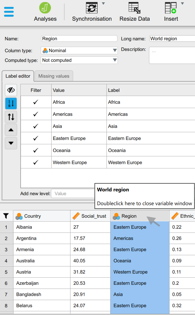
In the “Label editor”, we first deselect the “Automatically order labels by their value” (currently in blue) and with the up/down arrows we can move categories around. We can move “Western Europe” in the top position so that it will be the first category and as such set as the “reference” category in regression models:
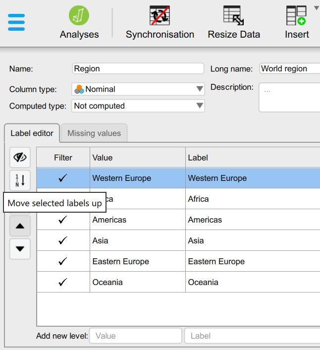
Once we perform this change and return to our regression in the Analyses window, we see that the output was already automatically updated:
Now all the Regoins listed in the Coefficients list are compared to “Western Europe”. We find that countries in all regions except Oceania are predicted to have smaller levels of Trust compared to Western Europe.
Task 5: Fit a linear regression model to assess the relationship between “social trust” and whether a country has a dominant “Protestant” population
Even through “Protestantism” appears in the dataset as a “Scale” type variable, we can move it to the “Factors” box and it will automatically be treated as a “Nomical” categorical variable; a small black star next to the variable type icon will signal that the variable was “forced” into behaving like a “Factor”:

When done, you should be seeing some of these outputs:
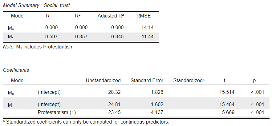
Questions
- What is the expected
Social_trustlevel of a country that does not have a dominant Protestant population? - What is the expected
Social_trustlevel of a country that has a dominant Protestant population? - How much higher or lower is the expected
Social_trustin a Protestant country compared to a non-protestant one?
The interpretation of the coefficients is exactly the same as in the previous case (Regions), with the exception that now we only have one category to compare against the “reference” because the Protestantism variable is naturally dichotomous/binary one, containing only two categories.
Because of this, we could treat Protestantism as a “Scale” type variable and enter it into the “Covariates” box instead, and still get the same coefficients because it would be treated as a theoretically infinite scale on which we only observe two data points in practice (0 as non-Protestant and 1 as Protestant), and so we can imagine a one-unit change on this scale as being a movement from the first category to the second.
The only differences in the output would be the naming of the variable and - more importantly - that Standardised coefficients would also be calculated and displayed. Because in this case we have not labelled the values themselves (the two categories of the Protestantism variable have not been given labels, just the values 0 and 1), the naming of the output is actually cleaner when treating Protestantism as a “scale” type variable. This is common practice for dichotomous/binary/“dummy”/indicator variables, where the variable name “indicates” the case coded as 1 (here “Protestantism”; in the case of a variable categorising biological sex, we could name the variable itself as female and code males as 0 and females as 1).
The output from a regression in which we treat Protestantism as a “Scale” variable would look something like this:
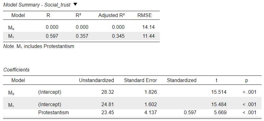
It is often easier to treat dichotomous/“dummy”/indicator variables as “Scale” for modelling purposes. We can then calculate meaningful mean values for them and to standardise them to make them comparable with the scales of the other variables in the model. If we examine the regression results presented by Delhey and Newton (2005) in their Table 3, we realise that they actually report “Standardised” coefficients, meaning that all the predictor variables had been standardised before entered into the regression model.
Exercise 3.4: “Predicting Cross-National Levels of Social Trust”
You should now be well-equipped to reproduce and interpret the main regression models reported on in Table 3 in Delhey and Newton (2005) . The authors were interested in identifying the strongest predictors of national-level social trust and tested the effect of several potential explanatory variable. They found five that proved statistically significant (more on this later in Workshop 5) and robust across different models, and our delhey&newton2005 dataset contains all the relevant variables to reproduce these results. We should note that the dataset was compiled from a variety of sources described by the original authors in their article, but it is not the original dataset used by the authors themselves, so we should expect some differences compared to the published results.2 Nevertless, the results should be robust enough to withhold some variability in the data.
In this exercise, you have free hand to reproduce the four highlighted models from the article’s Table 3:
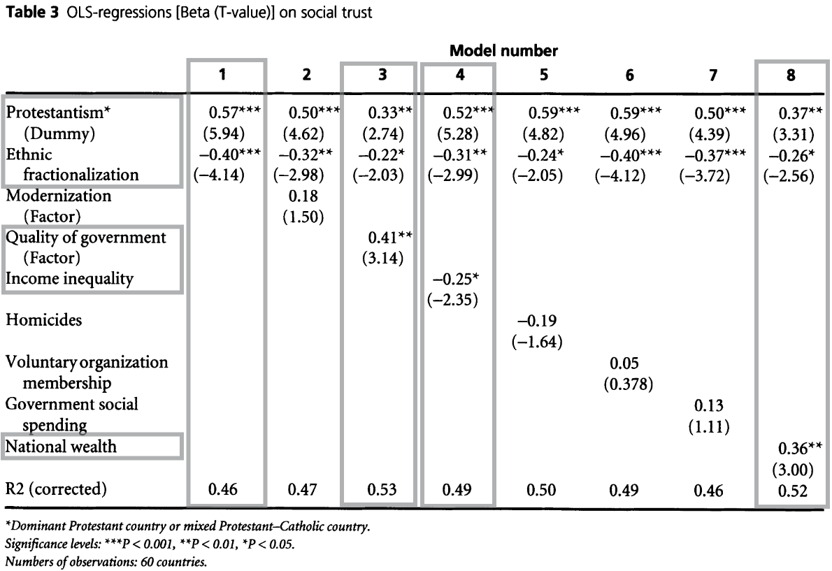
Questions
- Which coefficients in the JASP output are the ones that match the coefficients reported in the article? Note that there are likely some differences in the actual numbers, but they should be still recognisably close to the published ones.
- How do you interpret the results from these models?
- What limitations in the analysis can you think of? What criticisms can you formulate?
Exercise 3.5: Which of the assignment research questions could be addressed using a linear regression model?
Let’s look again at the assignment research questions. Some of these questions imply a dependent variable which is measured as a numeric scale or at least a long-ish (e.g. 7-point +) ordinal scale in one of the surveys we will use for the assignment (ESS10, WVS7, EVS2017). Other questions imply dependent variables that are more strictly categorical, and as such, we cannot model them using linear regression. For those, we may be able to apply another model type that better fits that kind of outcome variable (e.g. logistic regression), one of which we will be covering in Week 5.
In this exercise, explore the survey questionnaires (like we did in previous Workshops) to identify any available variables for answering one/some of the questions below, and check how the implied dependent variable was measured:
- Are religious people more satisfied with life?
- Are older people more likely to see the death penalty as justifiable?
- What factors are associated with opinions about future European Union enlargement among Europeans?
- Is higher internet use associated with stronger anti-immigrant sentiments?
- How does victimisation relate to trust in the police?
- What factors are associated with belief in life after death?
- Are government/public sector employees more inclined to perceive higher levels of corruption than those working in the private sector?
The best way to explore the available Assignment datasets and questionnaires is via the Data page of this site.
JASP solutions
Below you can download JASP files with solutions to some of the exercises in this worksheet:
References
Footnotes
By the way, a “quintile” (from the Latin word “quintus” for “five”) is simply a value that divides a scale into five equal parts - e.g. a scale of all the integers between 0 and 100 divided into five equal parts will contain 20 integers in each part, i.e. 100÷5↩︎
Some of the potentially most consequential sources of difference between the two datasets are the following: I could not find Ghana as a participating country in either the 1996 or 1990 World Values Survey; however, Malta was a participating country and also had useful measurements on all the other explanatory variables, so I have included it in the list of countries, making the dataset add up to 60, in line with the original sample size. Macro-economic data published by the World Bank or the OECD are often updated and corrected retrospectively, so if data for previous time periods are drawn form more recently published data releases, they may be slightly different than those available earlier. The categorisation of “Protestantism” is not described in too much detail by the authors, so it may be slightly different than the one done here (nonetheless, I have experimented with different possible options for coding it and the version included in the dataset was the most robust version). The finer details of the factor analysis used to compile the “Quality of government” scale were also not described by the authors, but the approach adopted here showed fit statistics that were close to those reported by the authors.↩︎